What is centrality in graphs?

Introduction

In this article we will understand what centrality is and show the most common measures of centrality. We will find out the centrality with various measures using the “igraph” package in R, and discuss the difference between such measures.

What is a graph?

First of all, a graph $G$ (a.k.a network) is made up of two sets: the vertex set $V(G)$ (set of vertices of $G$ ) and the edge set $E(G)$ . The vertices (a.k.a. nodes) are visually represented by small circles or dots. Each edge (a.k.a. link) joins two vertices, and this is represented by a line joining the respective two dots. If there is an edge joining two vertices, then it means that there is a relation between these two vertices. In real world analysis, a graph could be used to model various situations. Let’s give some examples.

Popular applications of graphs

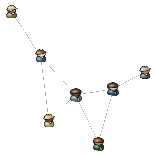
In social graphs, the vertices represent a group of people and edges model the presence of an acquaintance, friendship or working relationship between two persons. In transportation graphs, the vertices can represent geographic destinations or places and the edges can represent roads or routes. Other technology graphs can model the distribution of water and electricity, or telephone and internet connections. In information graphs, the vertices can represent books, scientific papers or websites and the edges can represent references, citations or hyperlinks.

Two types of Centralities

In graph theory centrality is defined as importance (or influence or priority). However this arises two questions: 1) What is “important” referring to? 2) How is importance defined? Let’s answer the first question. When we are comparing between graphs, we are giving a value of importance (centrality) to a whole graph. This is called graph centrality. On the other hand, when we have a graph we can analyse which vertices are more important by giving a value of importance (centrality) to each vertex. This is called point centrality. Hence we have two types of centralities. In what follows we will assume point centrality and answer the second question by showing various measure of centrality. For all these measures the exact value of centrality of a vertex is usually not relevant per se. What is more relevant is the ranking of the vertices according to the measure and the ratio of the centrality values of any pair of vertices. These computations are useful for the analysis and comparison of importance between vertices.

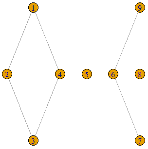
The followings is the R code that gives us a graph on which we will compute various centrality measures. First of all, it is required to load the package “igraph” which includes various in-built functions related to graph theory. The graph is constructed from a vector named “edges” which is a list of all the edges of the graph and by stating the number of vertices (9) in the function “graph”. The matrix “l” is a list of the Cartesian coordinates of the vertices which determine the layout of the graph on a 2D plane.

library(igraph)

edges <- c(1,2,1,4,2,3,2,4,3,4,4,5,5,6,6,7,6,8,6,9)
g<-graph(edges, 9,directed=FALSE) 
l<-matrix(c(1,1,0,0,1,-1,2,0,3,0,4,0,5,-1,5,0,5,1),nrow = 9,ncol=2,byrow=TRUE) #custom layout
plot(g,layout = l)

The following is the graph that we will use as example.

Degree Centrality

The $\bf{degree\ centrality}$ is the most basic and intuitive measure of centrality. Here each vertex gets its value of importance by calculating the total number of its neighbours (known as the degree of the vertex) and divided by the sum of degrees of all the vertices in the graph. Thus the degree centrality of a vertex $v\in V(G)$ is:

$\begin{equation*} C_D(v)=\frac{\rho_v}{2m} \end{equation*}$

where $\rho_v$ is the degree of vertex $v$ and $2m$ is equal to the sum of the degrees of all the vertices of $G$ . Hence the more neighbours a vertex has, the more it is considered to be important.

#Degree Centrality

degree_centrality<-degree(g)/sum(degree(g))
degree_centrality

par(mfrow=c(1,2))
plot(g,layout=l)
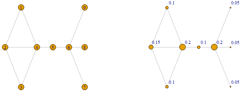
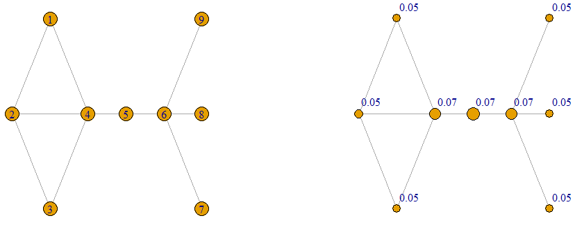
plot(g,vertex.label=round(degree(g)/sum(degree(g)),2),layout=l,vertex.label.dist=2.5,vertex.size=80*degree_centrality)

The labels of the graph on the right give the values of the centrality. The sizes of the vertices are proportional to the centrality value. Here vertices 4 and 6 have the largest degree centrality whilst the end-points 7, 8 and 9 share the lowest value.

Betweenness Centrality

The $\bf{betweenness\ centrality}$ of a vertex $v$ is the sum of the fraction of shortest paths between vertices $i$ and $j$ that pass through $v$ , over all vertex pairs $\lbrace i,j\rbrace$ , in which $i\neq j$ , and $i,j\neq v$ . The equation for betweenness centrality of a vertex $v\in V(G)$ is given by:

$\begin{equation*} C_B(v)=\sum_{i,j\in V(G),i\neq j, i,j\neq v}\frac{\sigma_{i,j}(v)}{\sigma_{i,j}}, \end{equation*}$

where $\sigma_{i,j}$ is the number of shortest paths from $i$ to $j$ and $\sigma_{i,j}(v)$ is the number of shortest paths from $i$ to $j$ passing through $v$ . Here a vertex is considered important if it lies in a good number of shortest paths between any two pair of vertices. In graphs that model the flow of information between its vertices, the removal of vertices with an associated high betweenness centrality seems to affect extremely the flow of information, assuming that the flow travels mostly through shortest paths.

#Betweenness Centrality

betweenness(g)

par(mfrow=c(1,2))
plot(g,layout=l)
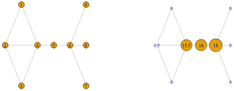
plot(g,vertex.label=betweenness(g),layout=l,vertex.size=2*betweenness(g))

Vertices 4, 5 and 6 have the highest betweenness centrality values. In fact these are the vertices whose removal would disconnect the graph and so are critical to the connectivity of the network. All paths between a vertex from $\lbrace 1, 2, 3\rbrace$ and a vertex from $\lbrace 7, 8, 9\rbrace$ go through the vertices 4, 5 and 6.

Closeness Centrality

The $\bf{closeness\ centrality}$ of a vertex measures how close a vertex is to the other vertices in the graph. This can be measured by reciprocal of the sum of the lengths of the shortest paths between the vertex and all other vertices in the graph. The equation for the closeness centrality of a vertex $v\in V(G)$ is given by:

$\begin{equation*} C_C(v)=\frac{1}{\sum_{i=1}^n d(v,i)}, \end{equation*}$

where $d(v,i)$ is the length of the shortest path between vertices $v$ and $i$ . For the case when the graph is not connected, only the shortest paths between the vertex and the other vertices in the same component are considered in the sum. Hence a vertex with a high closeness centrality seems to be close, in terms of distance, to the majority of the vertices in the graph.

#Closeness Centrality

closeness(g)

par(mfrow=c(1,2))
plot(g,layout=l)
plot(g,vertex.label=round(closeness(g),2),layout=l,vertex.label.dist=2.5,vertex.size=190*closeness(g))

The vertices 4, 5, 6 are “central” vertices in the graph and thus have the highest closeness centrality.

Eigenvector Centrality

An extension of the degree centrality is that of the $\bf{eigenvector\ centrality}$ , which was probably first proposed by Philip Bonacich in 1987. In the degree centrality, the importance of a vertex depends only on the number of its neighbours. However the eigenvector centrality takes into consideration the fact that vertices in the graph are usually not equally important. So, if a vertex is connected to a relatively small number of vertices which are considered to be very important, its eigenvector centrality might be higher than that of a vertex having a considerable number of neighbours of low importance. The eigenvector centrality of a vertex $v\in V(G)$ is given by:

$\begin{equation*} C_E(v)=({\bf x_1})_v, \end{equation*}$

where ${\bf x_1}$ is the eigenvector of unit length corresponding to the largest eigenvalue of the adjacency matrix of the graph and $({\bf x_1})_v$ is the $v^{\mbox{th}}$ entry of vector ${\bf x_1}$ . Hence one could determine the eigenvector centrality values of all the vertices by just computing this eigenvector.

#Eigenvector Centrality

eigenvector_centrality<-eigen_centrality(g)[[1]]
eigenvector_centrality

par(mfrow=c(1,2))
plot(g,layout=l)
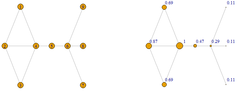
plot(g,vertex.label=round(eigenvector_centrality,2),layout=l,vertex.label.dist=2.5,vertex.size=18*eigenvector_centrality)

Here vertex 4 has the highest eigenvector centrality value. This the vertex that connects the complete subgraph with vertex set $\lbrace 1, 2, 3, 4\rbrace$ (called a clique) to the rest of the graph. In comparison to the degree centrality, in which vertices 4 and 6 have equal degree centrality value, here since vertex 4 is connected to vertices which are “more connected” and thus more important, and since vertex 6 is connected to some isolated vertices, vertex 4 has a higher eigenvector centrality value. In the betweenness centrality, vertex 6 is considered more important than vertex 4. This is a result of the fact that all the paths between vertices 7, 8 and 9 must pass through vertex 6.

Walk Centrality

A generalisation of the eigenvector centrality is the walk centrality. The walk centrality of a vertex $v$ in a graph $G$ is equal to the total number of walks in $G$ originating from vertex $v$ , where the walks of length $k$ are weighted by a factor ${\alpha}^k$ . Such a number decays as $k$ increases. Hence longer walks are given less weight in the formula of the walk centrality of a vertex. The parameter $\alpha$ is called the dampening factor, and $\alpha$ could take values from the interval $0<\alpha<\frac{1}{\lambda_1}$ where $\lambda_1$ is the largest eigenvalues of the graph. A larger value of $\alpha$ shows that the effect on the centrality across long walks decays slowly, and vice-versa. In this centrality measure, the larger the number of walks of a certain length $k$ from a vertex $v$ , the more the opportunity $v$ has to influence other vertices that are reached by walks of length $k$ . Similar measures have been proposed by L. Katz in 1953 and by P. Bonacich in 1987.

The formula for the walk centrality is:

$\begin{equation*} C_W(v;\alpha)=((\mathbb{I} - \alpha\mathbb{A})^{-1}{\bf j})_v. \end{equation*}$

where $\mathbb{A}$ is the adjacency matrix of the graph $G$ , $\mathbb{I}$ is the identity matrix and ${\bf j}$ is an all-one vector.

Let us consider our example. First we must find the range of values of $\alpha$ . Let’s first find the maximum eigenvalue $\lambda_1$ .

#Finding the maximum eigenvalue of the A

A<-as.matrix(get.adjacency(g))
max(eigen(A)[[1]])

In this case it is equal to 2.72273. Hence $\alpha$ can take an positive value less than $\frac{1}{\lambda_1}=0.372784$ . The following is a custom function, named “walk_centrality” that gives the walk centrality vector which is scaled (this avoids having extremely large values as $\alpha$ gets nearer to $\frac{1}{\lambda}$ ). The inputs of this function is the graph “g” and the value of $\alpha$ “alpha”.

walk_centrality<-function(g,alpha){w<-as.vector(solve(diag(vcount(g))-alpha*as.matrix(get.adjacency(g)))%*%rep(1,vcount(g)))
w/sqrt(sum(w^2))}

walkcentrality<-walk_centrality(g,0.1)

par(mfrow=c(1,2))
plot(g,layout=l)
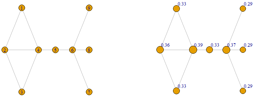
plot(g,vertex.label=round(walkcentrality,2),layout=l,vertex.label.dist=2.5,vertex.size=50*walkcentrality)

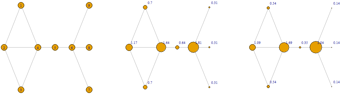
The following are three rankings of the vertices according to the walk centrality measure using three different values of $\alpha$ ‘s: 0.1, 0.2, 0.36. The smaller the value of $\alpha$ , the more the vertices have equal importance. The larger the value of $\alpha$ , the closer the walk centrality values are to the eigenvector centrality values. The labels on the graph on the top right, bottom left and bottom right are the walk centrality values when $\alpha=0.1, 0.2$ and 0.36 respectively.

Power Centrality

Here is the power centrality according to Phillip Bonacich. This measure calculates the power, authority or dominance of a vertex $v$ by considering the degrees of its neighbours. If a neighbour $w$ of $v$ has few neighbours, then $v$ is powerful on $w$ , and if on the other hand $w$ has lots of neighbours, the power of $v$ on $w$ is low. As an example in a network of friends, an individual X is powerful when having a number of friends having a low number of contacts. Suppose Y is one of these friends of X. It is very likely for Y to turn to X to interact, giving X power. In fact this measure was motivated by social networks modelling bargaining power.

The formula for the power centrality is:

$\begin{equation*} C_P(v;\alpha)=((\mathbb{I} - \alpha\mathbb{A})^{-1}\mathbb{A}{\bf j})_v. \end{equation*}$

where $\mathbb{A}$ is the adjacency matrix of the graph $G$ , $\mathbb{I}$ is the identity matrix, ${\bf j}$ is an all-one vector and $\alpha$ is the attenuation factor which lies in the interval $(-\frac{1}{\lambda_1},\frac{1}{\lambda_1})$ . When $\alpha$ is greater than 0, it means that a vertex is more powerful if its neighbours are more powerful. Hence this would become similar to the walk centrality. So we will focus on the case when $\alpha$ is smaller than 0, that is, when a vertex is more powerful if it has less powerful neighbours.

The following is the R code for the power centrality. Note that the “exponent” represents $\alpha$ . The power centrality output vector is automatically scaled in order to avoid entries of large magnitude.

power_centrality(g,exponent=-0.2)

par(mfrow=c(1,2))
plot(g,layout=l)
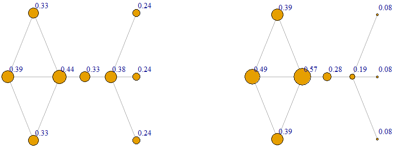
plot(g,vertex.label=round(power_centrality(g,exponent=-0.2),2),layout=l,vertex.label.dist=2.5,vertex.size=15*power_centrality(g,exponent=-0.2))

The following are two rankings of the vertices according to the power centrality measure using two different values of $\alpha$ ‘s: -0.1 and -0.2. Here vertex 6 has the most power due to its connection to the end-vertices 7, 8 and 9. On the other hand, these end-vertices have the least power due to their low degree.

Conclusion

The degree, betweenness, closeness, eigenvector, walk and power centrality measures are the most common point centrality measures for graphs. We have seen how different measures define what we mean by importance or central, in different ways. Thus the choice of centrality measure depends on what type of structure a graph is modelling. The ideas mentioned here are also extended to digraphs in which we have arcs instead of edges. An arc is an edge that has a direction. Arcs are represented by arrows going from one vertex to the other. Such algorithms include HITS and PageRank which are used to rank the importance of websites according the hyperlink structure.