How to generate any Random Variable (using R)

How to generate any random variable (using R)

Introduction

In this article we will explain and demonstrate two methods of generating a random variable. One of the methods requires the knowledge of the probability density function and the other method requires the cumulative distribution function. Nowadays software packages, including R, have in-built functions that generate random variables from well-known distributions like the normal, poisson, exponential etc…, in a direct way. However the advantage of knowing these two methods is that one will be able to generate random variables from any distribution including those that are not standard and not in-built in the statistical software. First both methods are explained, together with their advantages and limitations. Then both methods are coded in R in order to produce a sample derived from a custom distribution.

The Accept-Reject Method

This method generates realisations of a random variable $X$ using its probability density function $f(x)$ . Let $M$ be some real number greater than (or equal to) $f(x)$ for any possible value of $x$ . The choice of $M$ depends on the user and will always work as long as $M\geq f(x)$ . A number $u$ is generated randomly (uniformly) from the domain of $X$ . Now a test is done to see if the number $u$ will be accepted as part of our sample or else rejected (hence the name of this method). The number $u$ is accepted with probability $\frac{f(u)}{M}$ and rejected with probability $\frac{M-f(u)}{f(u)}$ .

The process of choosing a uniform random number from the domain of $X$ and deciding whether to accept it or not, is repeated on and on until the requested sample size is attained. Note that the greater the value of $f(u)$ , the greater the chance that $u$ is accepted as part of the sample. This ensure that histogram of the sample would have the shape of the probability density functions from which the realisations of the random variable are extracted.

The Analytical Inversion Method

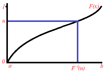
Let $X$ be a random variable having the cumulative distribution function $F(x)$ . The range of the function F(x) is [0,1]. Let $u$ be a random number (uniformly distributed) between 0 and 1. We include in our sample the value $x$ from the domain of $X$ , where $u=F(x)$ . The value of $x$ is obtained from the inverse of the cumulative distribution. We have $x=F^{-1}(u)$ . This process is repeated until the required sample size is obtained. This idea is derived from the result that if the random variable $U$ is uniformly distributed, $F^{-1}(U)$ (where $F^(-1)$ is the inverse cumulative distribution of $X$ ) has probability density function $f(x)$ .

Advantages and Limitations in the two methods

In the Analytical Inversion Method, every iteration in this process results in an additional one realisation of the random number $X$ . Hence the number of iterations is equal to the required sample size. In contrast to this, in the Accept-Reject Method, the number of iterations $n$ is greater than the sample size $S$ (because some generated values of $u$ are rejected). It can be shown that $S$ itself is a binomially distributed random variable with mean $\frac{n}{M(b-a)}$ and variance $n\frac{1}{M(b-a)}(1-\frac{1}{M(b-a)})$ , where $[a,b]$ is the domain of $X$ . Hence when computing $n$ iterations you expect to have a sample of size $\frac{n}{M(b-a)}$ .

Note that the Accept-Reject Method works only when the domain of $X$ is bounded. In fact, without loss of generality, suppose that $X$ is unbounded above and hence its domain is $[a,\infty)$ for some number $a$ . We cannot assign a uniform distribution over the interval $[a,\infty)$ which has infinite length. The Analytical Inverse Method is able to handle random variables with infinite domain size. However one must note that in some instances it might be hard to obtain an algebraic formula for the inverse-cumulative distribution function.

Worked Example

Let $X$ be a random variable with probability density function given by:

$f(x)=\begin{cases} \frac{3}{124}(6-x)^2 & 1\leq x\leq 5 \\ 0 & \mbox{otherwise}. \end{cases}$

The following is the cumulative distribution function of $X$ , which is derived from $f(x)$ through integration.

$F(x)=\begin{cases} 0 & x<0\\ \frac{1}{124}[(x-6)^3+125] & 1\leq x\leq 5 \\ 1 & x>1. \end{cases}$

The inverse cumulative function is given by:

$\begin{equation*} F^{-1}(x)=6+\sqrt[3]{124x-125}\mbox{ for } 0\leq x \leq 1 \end{equation}$

We would like to obtain a sample that follows this distribution. We will do this via the two methods, by coding in R. First of all, let us obtain a plot for the probability density function and the cumulative distribution function for this example, over the domain of $X$ which is $[1,5]$ .

library(ggplot2) 
library(cowplot)

x<-seq(1,5,0.1) #defining the range of X

#pdf
Curve<-3*(6-x)^2/124
Density<-data.frame(x,Curve)
plot1<-ggplot()+geom_line(data=Density,aes(x=x,y=Curve))+ scale_x_continuous(breaks = seq(1,5,by=1))+ylab("f(x)")+ggtitle("Probability Density Function")

#cdf
Curve<-((x-6)^3+125)/124
Cumulative<-data.frame(x,Curve)
plot2<-ggplot()+geom_line(data=Cumulative,aes(x=x,y=Curve))+ scale_x_continuous(breaks = seq(1,5,by=1))+ylab("F(x)")+ggtitle("Cumulative Distribution Function")

plot_grid(plot1, plot2)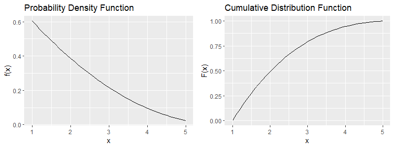

Let us start with the algorithm for the Accept-Reject Method. We will set $M$ to be $\frac{75}{124}$ . This is the maximum value of f(x) over the domain [1,5]. Thus the condition $f(x)<=M$ for all $x$ in the domain of $X$ is satisfied. The variable $S$ is the required sample size, initially set as an empty vector. The code involves a while loop that stops when the required sample size $S$ is reached. The code outputs a histogram of the sample.

#Accept-Reject Algorithm

S<-100 #sample size

M<-75/124
Sample<-c() #sample set

while(length(Sample)<S)
{u<-runif(1,1,5)
f<-3*(6-u)^2/124
if(runif(1,0,1)<=f/M){Sample<-c(Sample,u)}}
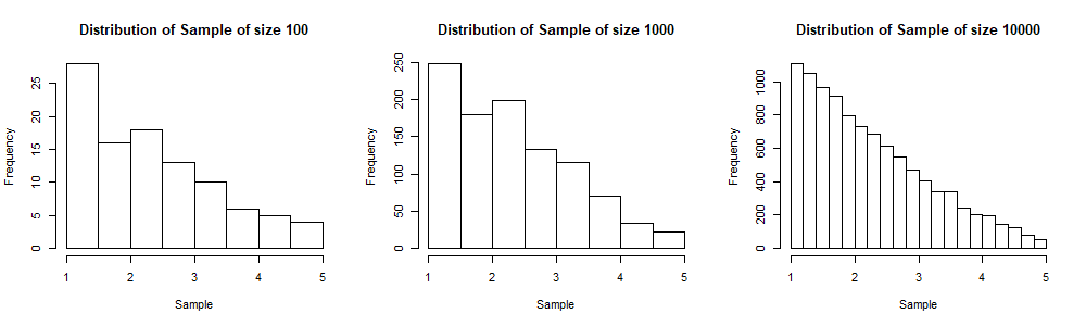
hist(Sample,main=paste("Distribution of Sample of size",as.character(S)))

We will display the histograms of three simulated samples, for sample sizes 100, 1,000 and 10,000 respectively. Note that as we increase the sample size, the shape of the histogram gets near to that of the probability density function $f(x)=\frac{3}{124}(6-x)^2$ (from which the sample is generated). In the three plots below, the sample of size 10,000 includes the sample of size 1,000 and the sample of size 1,000 includes the sample of size 100. This is done to visualise better the convergence of the shape of the sample distribution to the population distribution as the sample size increases.

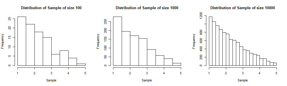
Next is the algorithm for the Analytical Inversion method. A number $u$ is selected randomly from the interval [0,1] and the value $F^{-1}(u)=6+\sqrt[3]{124u-125}$ is added to the sample.

#Analytical Inversion Algorithm

S<-100 #sample size

Sample<-c() #sample set
while(length(Sample)<S)
{u<-runif(1,0,1)
Sample<-c(Sample,6-(125-124*u)^(1/3))}
hist(Sample,main=paste("Distribution of Sample of size",as.character(S)))

The following three histograms correspond to three nested samples of sizes 100, 1,000 and 10,000 respectively. Again we see the distribution of the sample converging to the population distribution as the size increases.

Convergence of the two methods

We have already seen that the shape of the histogram converges to that of the probability density function, for both methods. Now let us picture what happens to the sample mean and sample standard deviation as the sample size increases, under both methods. We will compare the sample statistics to the population parameters. The population mean is given by:

$\begin{equation*} \begin{split} \mathbb{E}(X)&=\int_{1}^{5} x \frac{3}{124}(6-x)^2 dx\\ &=\frac{69}{31}\\ &\simeq 2.2258. \end{split} \end{equation*}$

The population variance is given by:

$\begin{equation*} \begin{split} \mbox{Var}(X)&=\int_{1}^{5} (x-\frac{69}{31})^2\frac{3}{124}(6-x)^2 dx\\ &=\frac{4188}{5(31^2)}. \end{split} \end{equation*}$

Thus the population standard deviation is given by:

$\begin{equation*} \mbox{sd}(X)=\frac{\sqrt{4188}}{31\sqrt{5}}\simeq 0.9336. \end{equation*}$

We will generate a random sample of 10,000 readings, and while the sample is gathered, at every step of 100 values, we record the sample mean and the sample standard deviation. Thus we can have a look at the convergences of these statistics to the population mean and standard deviation. The following is the code for the Accept-Reject Method. The vector “SampleSize” results in the sequence $100, 200,\cdots,10,000$ . The vectors “SampleMean” and “SampleSD” collects the data for the means and standard deviations of the sample at every new 100 realisations. This data is used to generate plots.

library(ggplot2)
library(cowplot)

S<-10000 #maximum sample size

M<-75/124
Sample<-c() #sample set

SampleSize<-c()
SampleMean<-c()
SampleSD<-c()

#simulation
while(length(Sample)<S)
{u<-runif(1,1,5)
f<-3*(6-u)^2/124
if(runif(1,0,1)<=f/M){Sample<-c(Sample,u)}

if(length(Sample)!=0 & length(Sample)%%100==0){if(length(Sample)>max(SampleSize)){SampleSize<-c(SampleSize,length(Sample));SampleMean<-c(SampleMean,mean(Sample));SampleSD<-c(SampleSD,sd(Sample))}}
}

#plots
Data<-data.frame(SampleSize=c(SampleSize,SampleSize),Mean=c(SampleMean,rep(69/31,length(SampleSize))),SD=c(SampleSD,rep((sqrt(4188)/(31*sqrt(5))),length(SampleSize))),Type=Type<-c(rep("Sample",length(SampleSize)),rep("Population",length(SampleSize))))
plot1<-ggplot()+geom_line(data=Data,aes(x=SampleSize,y=Mean,color = Type))+ scale_x_continuous(breaks =seq(0,10000,by=2000))+xlab("Sample Size")+ylab("Mean")+ggtitle("Convergence of Mean for Accept-Reject Method")
plot2<-ggplot()+geom_line(data=Data,aes(x=SampleSize,y=SD,color = Type))+ scale_x_continuous(breaks =seq(0,10000,by=2000))+xlab("Sample Size")+ylab("SD")+ggtitle("Convergence of St.Dev for Accept-Reject Method")

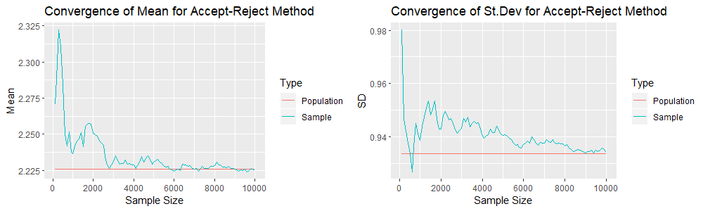
plot_grid(plot1, plot2)

The following are the resultant two plots of the sample means and standard deviations. Note that the red lines correspond to the population mean ( $\sim 2.2258$ ) and the population standard deviation (0.9336) respectively.

The same thing is done using the Analytical Inversion Method. The following is the R code.

library(ggplot2)
library(cowplot)

S<-10000 #maximum sample size

Sample<-c()

SampleSize<-c()
SampleMean<-c()
SampleSD<-c()

#simulation
while(length(Sample)<S)
{u<-runif(1,0,1)
Sample<-c(Sample,6-(125-124*u)^(1/3))
if(length(Sample)!=0 & length(Sample)%%100==0){SampleSize<-c(SampleSize,length(Sample));SampleMean<-c(SampleMean,mean(Sample));SampleSD<-c(SampleSD,sd(Sample))}
}

#plots
Data<-data.frame(SampleSize=c(SampleSize,SampleSize),Mean=c(SampleMean,rep(69/31,length(SampleSize))),SD=c(SampleSD,rep((sqrt(4188)/(31*sqrt(5))),length(SampleSize))),Type=Type<-c(rep("Sample",length(SampleSize)),rep("Population",length(SampleSize))))
plot1<-ggplot()+geom_line(data=Data,aes(x=SampleSize,y=Mean,color = Type))+ scale_x_continuous(breaks =seq(0,10000,by=2000))+xlab("Sample Size")+ylab("Mean")+ggtitle("Convergence of Mean for Inversion Method")
plot2<-ggplot()+geom_line(data=Data,aes(x=SampleSize,y=SD,color = Type))+ scale_x_continuous(breaks =seq(0,10000,by=2000))+xlab("Sample Size")+ylab("SD")+ggtitle("Convergence of St.Dev for Inversion Method")

plot_grid(plot1, plot2)

We have the following two plots for the sample means and standard deviations.

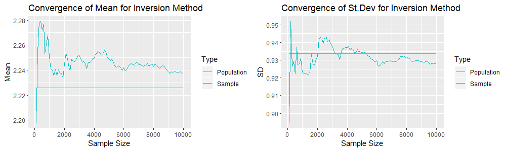
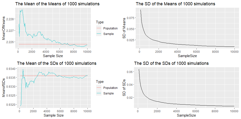
We see that the convergence of the sample mean and standard deviation seems to be weaker here. However we must note that we have a simulation of one sample of 10,000 realisations for each method. Thus we are comparing one sample with one sample, and thus the variability might be a result of sampling randomness and not because one method is superior to the other. Hence we will compare the sample means and standard deviation when we compute 1000 simulations for each method. The R code builds on the previous ones and will be given in the appendix below, because of their length. The following are 4 plots that result from the Accept-Reject Method. Recall that one simulation gives us a mean value for each sample of size $100, 200, \cdots,10000$ . Thus, since we have 1000 simulations, we have 1000 mean values for each sample of size $100, 200, \cdots,10000$ . We compute the mean of these 1000 mean values and obtain the first plot in the grid. We see that mean of the mean values is getting nearer to the population mean (represented by the red line). We compute the standard deviation of these 1000 mean values and obtain the second plot in the grid (first row, second column). This graph is converging to zero which shows that the variability of the sample means is decreasing as the sample size increases and confirms convergence. We also compute the mean and standard deviation of the 1000 standard deviation values for each sample of size $100, 200, \cdots,10000$ to obtain the third and fourth plot. These confirm the convergence of the mean of the standard deviations to the population standard deviation as the sample size increases.

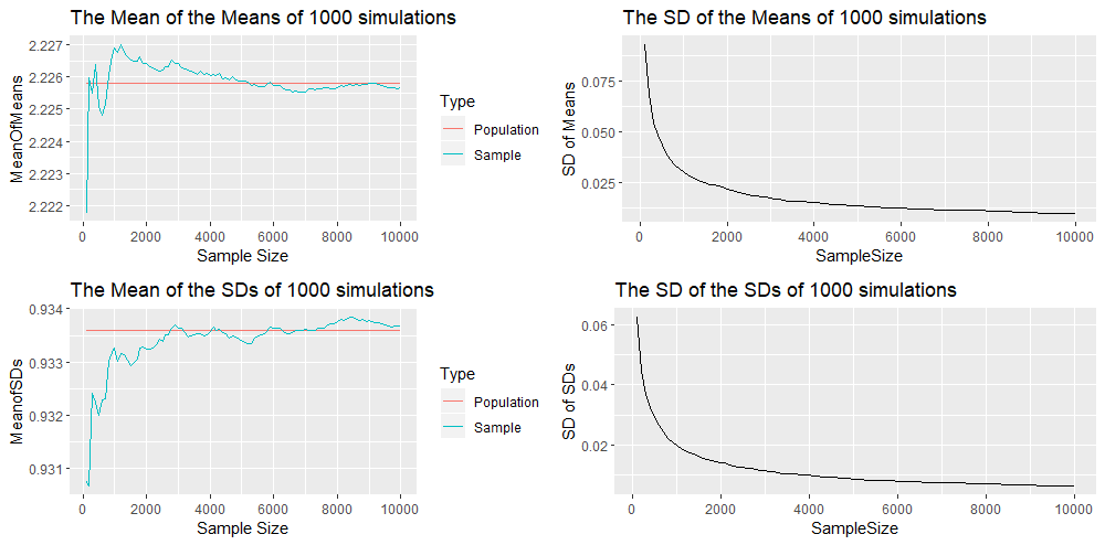
We also have the output obtained by using the Analytical Inversion Method. Again here the plots show the convergence of the sample mean and sample standard deviation to the population mean and population standard deviation. These plots do not hint that one method of generating random numbers is superior than the other.

Conclusion

We have described two methods of generating random numbers, together with their advantages and limitations. We have applied both methods to obtain samples from a custom distribution and test their convergence by repeating a simulation a thousand times. No method seems to be superior to the other in terms of speed of convergence, when tested on our custom distribution.

Appendix

The following is the R code related to the convergence of the Accept-Reject Method.

library(ggplot2)
library(cowplot)

N<-1000 #number of simulations

S<-10000 #maximum sample size
M<-75/124

MeanData<-data.frame() #will contain data of the means of all simulations
SDData<-data.frame() #will contain data of the standard deviations of all simulations


for (i in 1:N)
{Sample<-c() #sample set

SampleSize<-c()
SampleMean<-c()
SampleSD<-c()


while(length(Sample)<S)
{u<-runif(1,1,5)
f<-3*(6-u)^2/124
if(runif(1,0,1)<=f/M){Sample<-c(Sample,u)}

if(length(Sample)!=0 & length(Sample)%%100==0){if(length(Sample)>max(SampleSize)){SampleSize<-c(SampleSize,length(Sample));SampleMean<-c(SampleMean,mean(Sample));SampleSD<-c(SampleSD,sd(Sample))}}
}

MeanData<-rbind(MeanData,SampleMean)
SDData<-rbind(SDData,SampleSD)
}

MeanOfMeans<-c()
for(i in 1:ncol(MeanData)){MeanOfMeans<-c(MeanOfMeans,mean(MeanData[,i]))}
SDOfMeans<-c()
for(i in 1:ncol(MeanData)){SDOfMeans<-c(SDOfMeans,sd(MeanData[,i]))}

MeanOfSDs<-c()
for(i in 1:ncol(SDData)){MeanOfSDs<-c(MeanOfSDs,mean(SDData[,i]))}
SDOfSDs<-c()
for(i in 1:ncol(SDData)){SDOfSDs<-c(SDOfSDs,sd(SDData[,i]))}


Data1<-data.frame(SampleSize=c(SampleSize,SampleSize),MeanOfMeans=c(MeanOfMeans,rep(69/31,length(SampleSize))),MeanOfSDs=c(MeanOfSDs,rep((sqrt(4188)/(31*sqrt(5))),length(SampleSize))),Type=Type<-c(rep("Sample",length(SampleSize)),rep("Population",length(SampleSize))))
Data2<-data.frame(SampleSize,SDOfMeans,SDOfSDs)

plot1<-ggplot()+geom_line(data=Data1,aes(x=SampleSize,y=MeanOfMeans,color = Type))+ scale_x_continuous(breaks =seq(0,10000,by=2000))+xlab("Sample Size")+ylab("MeanOfMeans")+ggtitle("The Mean of the Means of 1000 simulations")
plot2<-ggplot()+geom_line(data=Data2,aes(x=SampleSize,y=SDOfMeans))+ scale_x_continuous(breaks = seq(0,10000,by=2000))+ylab("SD of Means")+ggtitle("The SD of the Means of 1000 simulations")

plot3<-ggplot()+geom_line(data=Data1,aes(x=SampleSize,y=MeanOfSDs,color = Type))+ scale_x_continuous(breaks =seq(0,10000,by=2000))+xlab("Sample Size")+ylab("MeanofSDs")+ggtitle("The Mean of the SDs of 1000 simulations")
plot4<-ggplot()+geom_line(data=Data2,aes(x=SampleSize,y=SDOfSDs))+ scale_x_continuous(breaks = seq(0,10000,by=2000))+ylab("SD of SDs")+ggtitle("The SD of the SDs of 1000 simulations")

plot_grid(plot1, plot2,plot3,plot4,ncol=2)

The following is the R code related to the convergence of the Analytical Inversion Method.

library(ggplot2)
library(cowplot)

N<-1000 #number of simulations

S<-10000 #maximum sample size

MeanData<-data.frame() #will contain data of the means of all simulations
SDData<-data.frame() #will contain data of the standard deviations of all simulations

for(i in 1:N)
{
Sample<-c()

SampleSize<-c()
SampleMean<-c()
SampleSD<-c()

while(length(Sample)<S)
{u<-runif(1,0,1)
Sample<-c(Sample,6-(125-124*u)^(1/3))
if(length(Sample)!=0 & length(Sample)%%100==0){SampleSize<-c(SampleSize,length(Sample));SampleMean<-c(SampleMean,mean(Sample));SampleSD<-c(SampleSD,sd(Sample))}
}

MeanData<-rbind(MeanData,SampleMean)
SDData<-rbind(SDData,SampleSD)

}

MeanOfMeans<-c()
for(i in 1:ncol(MeanData)){MeanOfMeans<-c(MeanOfMeans,mean(MeanData[,i]))}
SDOfMeans<-c()
for(i in 1:ncol(MeanData)){SDOfMeans<-c(SDOfMeans,sd(MeanData[,i]))}

MeanOfSDs<-c()
for(i in 1:ncol(SDData)){MeanOfSDs<-c(MeanOfSDs,mean(SDData[,i]))}
SDOfSDs<-c()
for(i in 1:ncol(SDData)){SDOfSDs<-c(SDOfSDs,sd(SDData[,i]))}


Data1<-data.frame(SampleSize=c(SampleSize,SampleSize),MeanOfMeans=c(MeanOfMeans,rep(69/31,length(SampleSize))),MeanOfSDs=c(MeanOfSDs,rep((sqrt(4188)/(31*sqrt(5))),length(SampleSize))),Type=Type<-c(rep("Sample",length(SampleSize)),rep("Population",length(SampleSize))))
Data2<-data.frame(SampleSize,SDOfMeans,SDOfSDs)

plot1<-ggplot()+geom_line(data=Data1,aes(x=SampleSize,y=MeanOfMeans,color = Type))+ scale_x_continuous(breaks =seq(0,10000,by=2000))+xlab("Sample Size")+ylab("MeanOfMeans")+ggtitle("The Mean of the Means of 1000 simulations")
plot2<-ggplot()+geom_line(data=Data2,aes(x=SampleSize,y=SDOfMeans))+ scale_x_continuous(breaks = seq(0,10000,by=2000))+ylab("SD of Means")+ggtitle("The SD of the Means of 1000 simulations")

plot3<-ggplot()+geom_line(data=Data1,aes(x=SampleSize,y=MeanOfSDs,color = Type))+ scale_x_continuous(breaks =seq(0,10000,by=2000))+xlab("Sample Size")+ylab("MeanofSDs")+ggtitle("The Mean of the SDs of 1000 simulations")
plot4<-ggplot()+geom_line(data=Data2,aes(x=SampleSize,y=SDOfSDs))+ scale_x_continuous(breaks = seq(0,10000,by=2000))+ylab("SD of SDs")+ggtitle("The SD of the SDs of 1000 simulations")

plot_grid(plot1, plot2,plot3,plot4,ncol=2)