Which Multiple Comparison Test to use for ANOVA?

Which Multiple Comparison Test to Use After Anova?

Introduction

Suppose that we fit a one-way ANOVA model to a data. Let $v$ be the number of treatment levels. Hence the fitted ANOVA model equation is given by $y_{it}=\mu+\tau_i+\epsilon_{it}$ where $t=1,2,\cdots,r_i$ and $i=1,2,\cdots,v$ . Multiple comparison tests are used to find confidence intervals for a combination of contrasts or treatment means, given a required simultaneous confidence level. For example, we would like to find confidence intervals for the contrasts $\mu_1-\mu_2$ and $\mu_1-\mu_3$ and the probability that these two intervals are both true is 95%, that is, the simultaneous confidence level is 95%.

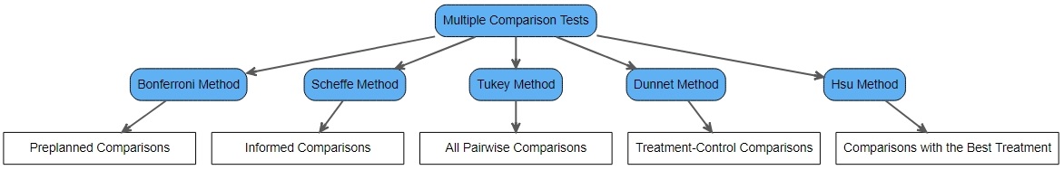
We are going to consider five multiple comparison test methods, each of them have their own particular use. Each method will be described in more details below.

Multiple Comparison Tests for ANOVA

Recall that a contrast is a linear combination of the $\tau_i$ ‘s: $\sum_{i=1}^{v}c_i\tau_i$ where each $c_i\in\mathbb{R}$ such that $\sum_{i=1}^{v}c_i=0$ . For example, $\tau_1-\tau_2$ is a contrast because it can be written in the form $\sum_{i=1}^{v}c_i\tau_i$ where $c_1=1$ , $c_2=-1$ and $c_i=0$ otherwise. The confidence interval of $\tau_1-\tau_2$ gives us the confidence interval for the difference between the effects of treatment levels 1 and 2.

Bonferroni Method

The Bonferroni Method is used only for pre-planned contrasts and means. This means that we would know the list of contrasts for which to find their confidence interval, before looking at the results of the data or before performing the ANOVA test. Thus we are not using the data and its results to help us identity the contrasts or means for which to compute the confidence interval.

Recall that the $100(1-\alpha)$ % two-tailed confidence level for a contrast $\sum_{i=1}^{v}c_i\tau_i$ is given by:

$\begin{equation*} \sum_{i=1}^{v}c_i \bar{y}_{i.}- t_{n-v,\frac{\alpha}{2}}\sqrt{MSE\sum_{i=1}^{v}\frac{c_i^2}{r_i}}\leq\sum_{i=1}^{v}c_i\tau_i\leq\sum_{i=1}^{v}c_i \bar{y}_{i.}+ t_{n-v,\frac{\alpha}{2}}\sqrt{MSE\sum_{i=1}^{v}\frac{c_i^2}{r_i}}, \end{equation*}$

where $\bar{y}_{i.}$ is the mean response of the subjects assigned treatment level $i$ , $n$ is the sample size, $MSE$ is the Mean Square Error found from the data by computing $\frac{1}{n-v}\sum_{i=1}^{v}\sum_{t=1}^{r_i}(y_{it}-\bar{y}_{i.})^2$ and $t_{n-v,\frac{\alpha}{2}}$ is percentile of the $t$ -distribution with $n-v$ degrees of freedom corresponding to a right-tail probability of $\frac{\alpha}{2}$ .

Bonferroni’s method is based on the general probability result that for any collection of sets $A_1,A_2,\cdots,A_k$ , $\mathbb{P}[\bigcup_{j=1}^k A_j]\leq \sum_{j=1}^k \mathbb{P}[A_j]$ . Suppose that we have $m$ such intervals, and we would like that such intervals are significantly correct with probability $1-\alpha$ . Assume that each individual interval is correct with probability $1-\beta$ .

$\begin{equation*} \begin{split} & \ \ \mathbb{P}[\mbox{all }m\mbox{ intervals are correct}]\\ &=1-\mathbb{P}[\mbox{at least one of the }m\mbox{ intervals is incorrect}]\\ &=1-\mathbb{P}[\bigcup_{j=1}^{m}\mbox{interval }j\mbox{ is incorrect} ]\\ &\geq 1-\sum_{j=1}^m\mathbb{P}[\mbox{interval }j\mbox{ is incorrect} ]\\ &= 1-\sum_{j=1}^m \beta\\ &=1-m \beta \end{split} \end{equation*}$

Let $m\beta=\alpha$ , that is, $\beta=\frac{\alpha}{m}$ . Hence having $m$ confidence intervals each having a confidence level of $(1-\frac{\alpha}{m})$ ensures a simultaneous confidence level of at least $1-\alpha$ . Each individual confidence interval for a contrast is thus given by:

$\begin{equation*} \sum_{i=1}^{v}c_i \bar{y}_{i.}- t_{n-v,\frac{\alpha}{2m}}\sqrt{MSE\sum_{i=1}^{v}\frac{c_i^2}{r_i}}\leq\sum_{i=1}^{v}c_i\tau_i\leq\sum_{i=1}^{v}c_i \bar{y}_{i.}+ t_{n-v,\frac{\alpha}{2m}}\sqrt{MSE\sum_{i=1}^{v}\frac{c_i^2}{r_i}}, \end{equation*}$

Note that in the trivial case when $m=1$ , the Bonferroni intervals are the same as the individual interval. When $m>1$ , the simultaneous confidence intervals with combined $\alpha$ signifincance level are obviously wider than the individual confidence intervals with individual $\alpha$ signifincance level.

Scheffe’s Method

Suppose that we compute the mean of each treatment level and possibly perform a one-way ANOVA. We would get an idea of the difference in effects (or lack of it) from the treatment levels. This would help us determine which contrasts are interesting for our study and for which we would like to find their confidence interval. Here we call such comparisons “Informed Comparisons” because the data is helping us choose the contrasts of interest. In this case, we should opt for Scheffe’s Method instead of Bonferroni’s Method. In contrast to the Bonferroni intervals, the Scheffe intervals do not depend on the number of intervals $m$ . This is based on the fact that any contrast can be written as a linear combination of the (treatment-control) contrasts: $\tau_2-\tau_1,\tau_3-\tau_1,\cdots,\tau_v-\tau_1$ . In fact:

$\begin{equation*} \begin{split} \sum_{i=1}^{v}c_i\tau_i&=c_1\tau_1+\sum_{i=2}^v c_i \tau_i\\ &=c_1\tau_1+c_2\tau_2+\cdots+c_v\tau_v+\sum_{i=2}^v c_i (\tau_i-\tau_1)\\ &=\sum_{i=2}^v c_i (\tau_i-\tau_1)\mbox{ (since }\sum_{i=1}^{v}c_i=0). \end{split} \end{equation*}$

The Scheffe confidence intervals for contrasts giving a simultaneous confidence level of $1-\alpha$ is given by:

$\begin{equation*} \sum_{i=1}^{v}c_i \bar{y}_{i.}- \sqrt{(v-1)F_{v-1,n-v,\alpha}}\sqrt{MSE\sum_{i=1}^{v}\frac{c_i^2}{r_i}}\leq\sum_{i=1}^{v}c_i\tau_i\leq\sum_{i=1}^{v}c_i \bar{y}_{i.}+ \sqrt{(v-1)F_{v-1,n-v,\alpha}}\sqrt{MSE\sum_{i=1}^{v}\frac{c_i^2}{r_i}}, \end{equation*}$

where $F_{v-1,n-v,\alpha}}$ is the percentile value of the $F$ -distribution with $d_1=v-1$ and $d_2=n-v$ and right-tail probability of $\alpha$ .

Tukey’s Method

Tukey’s Method is used in order to find confidence intervals for all pairwise mean comparisons. Thus we will be finding $\binom{v}{2}$ confidence intervals for the following contrasts: $\tau_1-\tau_2,\tau_1-\tau_3,\cdots,\tau_{v-1}-\tau_{v}$ . Note that Tukey’s method provides narrower intervals than Bonferroni’s or Scheffe’s Method when considering exactly all the pairwise comparisons. Hence in such case Tukey’s Method should preferred.

The Tukey confidence interval for contrast $\tau_k-\tau_s$ where $k\neq s$ that gives a simultaneous confidence level of at least $1-\alpha$ is given by:

$\begin{equation*} \bar{y}_{k.}-\bar{y}_{s.}-\frac{q_{v,n-v,\alpha}}{\sqrt{2}}\sqrt{MSE(\frac{1}{r_k}+\frac{1}{r_s})}\leq\tau_k-\tau_s\leq\bar{y}_{k.}-\bar{y}_{s.}+\frac{q_{v,n-v,\alpha}}{\sqrt{2}}\sqrt{MSE(\frac{1}{r_k}+\frac{1}{r_s})}, \end{equation*}$

where $q_{v,n-v,\alpha}$ is the percentile of the Studentized range distribution with parameters $v$ (number of groups) and $n-v$ (degrees of freedom), corresponding to a right-tail probability of $\alpha$ .

Dunnett’s Method

Suppose that we have one of the treatment levels which has a particular significance to the study. This is labelled as the “control”. For example, in practise the control could be a placebo, whereas the remaining treatments are different versions of drug developed by a pharmaceutical company. Dunnett’s Method is used to compare the control to all of the other treatments. W.l.o.g. let us say that the control is the first treatment level. Hence in Dunnett’s method we find $v-1$ confidence levels for the contrasts: $\tau_1-\tau_2,\tau_1-\tau_2,\cdots,\tau_1-\tau_v$ . The confidence intervals found by Dunnett’s Method are narrower than those provided by Bonferroni’s, Scheffe’s or Tukey’s method, in the case of treatment-control contrasts. Hence in such case Dunnett’s Method is preferred. The confidence intervals in this method are based on the multivariate $t$ -distribution. The Dunnett confidence interval for contrast $\tau_i-\tau_1$ giving a simultaneous confidence level of $1-\alpha$ is given by:

$\begin{equation*} \bar{y}_{k.}-\bar{y}_{s.}-\lvert t\rvert^{(0.5)}_{v-1,n-v,\alpha}\sqrt{MSE(\frac{1}{r_k}+\frac{1}{r_s})}\leq\tau_k-\tau_s\leq\bar{y}_{k.}-\bar{y}_{s.}+\lvert t\rvert^{(0.5)}_{v-1,n-v,\alpha}\sqrt{MSE(\frac{1}{r_k}+\frac{1}{r_s})}, \end{equation*}$

where $\lvert t\rvert^{(0.5)}_{v-1,n-v,\alpha}$ is the upper critical value for the maximum of the absolute values of a multivariate $t$ -distribution with correlation 0.5 and $n-v$ error degrees of freedom, corresponding to a right-tail probability of $\alpha$ .

Hsu’s Method

In Hsu’s method, $v$ confidence intervals are computed corresponding to a comparison between each treatment with the best of the other treatments (the treatment with the highest mean). If the resultant confidence interval is positive (contains no negative values), then the treatment is declared as the best treatment. If the resultant confidence interval is negative (contains no positive values), then the treatment is declared as not the best treatment. For equal treatment level sizes $r$ , the confidence interval which gives a simultaneous confidence level of $1-\alpha$ , corresponding to the comparison between treatment $i$ and the best of the other treatments, is given by:

$\begin{equation*} \bar{y}_{i.}-\max_{j\neq i}(\bar{y}_{i.})-t_{v-1,n-v,\alpha}^{(0.5)}\sqrt{MSE(\frac{2}{r})}\leq\tau_i-\max_{j\neq i} (\tau_j)\leq\bar{y}_{i.}+\max_{j\neq i}(\bar{y}_{i.})-t_{v-1,n-v,\alpha}^{(0.5)}\sqrt{MSE(\frac{2}{r})}, \end{equation*}$

where $t_{v-1,n-v,\alpha}^{(0.5)}$ is the precentile of the maximum of a multivariate $t$ -distribution with correlation 0.5 and $n-v$ degrees of freedom corresponding to a right-tail probability of $\alpha$ .

References

Design and Analysis of Experiments by Dean, Voss and Draguljic