The Mathematics behind portfolio VAR
Introduction
In this article we define VaR and give a brief overview of how it is used to quantify the risk of a portfolio. We will then go into a step-by-step mathematical derivation of VaR, whilst highlighting and discussing the various assumptions used along the way. The awareness of such assumptions is important to ensure reliable results and the use appropriate of models in order to avoid underestimation of risk.
Definition of VaR
Suppose that we have a portfolio of assets. Each asset has an associated price which changes from one time unit to the next. Hence the total value of the portfolio changes from one time unit to the next. The time unit could be a day, 5-day period, 1 week, 1 month, and so on. The choice of the time unit depends on how the historic data of prices is presented and the time horizon of the VaR calculation (as we shall see).
The term VaR stands for Value-At-Risk and has an associated time horizon and level of confidence. Let us say that the time horizon is 1 time unit for now. An  1-time unit VaR is the value
  by which with a level of confidence (or probability) of , the value of the loss suffered during 1 time unit would be not be greater than . As an example, if the 95% 5-day VaR is €100,000, then with a level of confidence of 95% , it is expected that the loss suffered during a 5-day period will not be greater than €100,000.
Consider the 1-time unit portfolio rate of return  defined by the percentage change in the value of the portfolio from one time point to the next. Suppose that we know the distribution of the . Let
  be the the value of
 ![\mathbb{P}[R\geq r]=\alpha](https://datasciencegenie.com/wp-content/ql-cache/quicklatex.com-a14c58c5aea6203b2fdc13b79e24ae2f_l3.png "Rendered by QuickLaTeX.com") . This means that the 1-time unit rate of return of the portfolio will be greater than ,
. This means that the 1-time unit rate of return of the portfolio will be greater than ,  of the time.
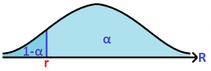
Then the 1-time unit VaR is equal to  , where
  is the total value of the portfolio.
Derivation of VaR
Suppose we have a portfolio of  assets. Let
  . Let
. Let  be the number of units of asset
  . Let
. Let  be the price of each unit of asset . Let
  be the total value of asset . Hence
  . Let
. Let  be the rate of return from asset during one time unit and let
  be the return from asset . Hence we have
  .
.
The portfolio can be described by the set  . Let the total current value of the portfolio be , where
  . The total return on the portfolio
  during one time unit is the sum of the return from each asset present in the portfolio. Thus
  . Finally the rate of return on the whole portfolio is given by:

where  for
for  and represents the weight of asset in the portfolio at the current time.
For every , let be a random variable with mean  and variance
  (not to be confused with VaR which represents the Value-At-Risk).
Then the mean  of the portfolio rate of return is given by:

and the variance  of the portfolio rate of return is given by:

where  is the covariance between and
  .
.
Hence is a random variable with mean and variance , given in terms of the means, variance and covariances of  . In order to characterise completely, we need to know the values of and , and also its distribution function.
Estimating the mean of the portfolio return and its variance
It is common practise that a series of prices is gathered for each asset over a time horizon common for all assets. Then the percentage change of a price of an asset, from one time unit to the next is the rate of return for that asset at that particular time interval. Hence a series of rates of return is obtain for each asset in the portfolio. The sample mean and the sample variance of each of these series are taken to be estimates of  and
and  .
.
Hence it is assumed that the means and the variances are independent of time. So time should not have any effect on the means and variances (no heteroscedasticity). In the case when the mean is increasing over the time horizon of the historic data, the risk is overestimated and vice-versa. In the case when the variance of the rates of return is increasing over the time horizon of the historic data, the risk is underestimated, and vice-versa. So one must check that the means and variances are more or less constant over the period of study.
Moreover the sample covariances between the series of rates of return are taken to be estimates of the covariances between the ‘s. Here it is assumed that the correlation structure is uniform over the values of the ‘s. Consider for example the case of positively correlated series (of rates of return). It is assumed that the correlation when the ‘s are positive is the same as that when the ‘s are negative. In the case when the correlation is higher when the ‘s are negative, the risk is underestimated.
Estimating the distribution of
It is common practise that each (for  ) is assumed to be normally distributed. In the case where the actual distribution is symmetric but has fatter tails than the normal distribution (positive excess kurtosis), the risk is underestimated, and vice-versa. This is known as kurtosis risk. In the case of an actual distribution which is skewed to the left (negatively skewed), there is underestimation of risk and vice-versa. This is known as skewness risk.
When we assume that each follows the normal distribution and moreover that the joint distribution of the ‘s is the multivariate normal distribution, then since is a linear combination of the ‘s, itself is normally distributed with mean and variance  , estimated as described above.
Estimating the 1-time unit VaR
We would like to find such that . We have:
![\begin{equation*}\begin{split}\mathbb{P}[R\geq r]&=\alpha\\\mathbb{P}[\frac{R-\mathbb{E}(R)}{\sqrt{\mbox{Var}(R)}}\geq \frac{r-\mathbb{E}(R)}{\sqrt{\mbox{Var}(R)}}]&=\alpha\end{split}\end{equation*}](https://datasciencegenie.com/wp-content/ql-cache/quicklatex.com-0c16f7c4a30d8a9e9bf35b5c2de2ad71_l3.png "Rendered by QuickLaTeX.com")
The random variable  follows the standard normal distribution (since is assumed to follow the normal distribution). Hence
  where
where  is the
  -score with probability
  . Therefore:

The  VaR is given by:

Sometimes when the value of is very small, it is assumed that  . This simplifies the VaR equation even further to just:

Extending to the  -time unit VaR
The 1-time unit  VaR could be extended to -time units VaR. Let
  be the portfolio rate of return over time units. In this case, the distribution of the portfolio logarithmic rate of return
  is calculated and used as a proxy of the distribution of .
For  , let
, let  be the rate of return during the
  time unit. Then:

Let us find the expected value and the variance fo the random variable .
Approximating  and
and 

since
 are identically distributed 1 time unit portfolio logarithmic rates of return.
Recall that the Maclaurin series of  . When the value of
  is small, we have the approximation
  , which we shall refer to as the “Maclaurin approximation”. By using the Maclaurin approximation on the formula for the expected value, we obtain:

Consider now the variance.

It is assumed that are not correlated, that is, there is no serial correlation present. Hence, in particular, situations in which a negative rate of return in one time point triggers a negative return in the time point, violates this assumption. By assuming that there is no serial correlation, the variance of the logarithmic rate of return reduces to:

and moreover

since are identically distributed 1 time unit portfolio logarithmic rates of return. This is the well-known square root of time rule because here the standard deviation of the logarithmic rate of return over a period of units is equal to the standard deviation of the logarithmic rate of return over one time unit multiplied by  (where is the time).
By the Maclaurin approximation, the formula for the variance reduces to

Approximate distribution of
If and each  is approximated by the Maclaurin approximation in the equation
  , and carry on with the assumption that the portfolio rate of return is normally distributed, then we assume that is normally distributed with mean
  and variance
  .
.
Hence the -time units VaR is  . Again, if is small and assumed to be zero, the VaR would reduce to
  .
.
Conclusion
We have gone through the mathematical derivation on the VaR equation for 1 time unit and for larger time horizons. The assumptions taken at each steps are highlighted. This is important for the risk manager to be aware of the assumptions being made and to make sure that the movement in the prices do not violate such assumptions. This will ensure that the portfolio risk is not underestimated and that the results are reliable.