Simulating a dynamic model
Introduction
In this article we are going to define what next event simulation is and adequate systems on which this simulation method could be performed. An example of a dynamic model is defined, on which the idea of the simulation is explained in detail and performed. Various results are obtain about the system. These are used to understand more the operational state of the system and provide insights on how the quality, efficiency and/or profitability of the system could be improved. The code in R which generates the simulation and the statistics on the system is provided. Finally the advantages of using simulation and Next Event Simulation are discussed.
What is Next Event Simulation?
Next event simulation is a method of simulation used when the state of the system being modelled changes at particular time points by the occurrence of some events. The state of the system remains constant until the next event happens. Hence the term next event simulation. The model simulates the next event and its timing and then records it. From knowing the state of the system, one could then generate informative results about the system. Since the state of the system is changing over time, the model of this system is called dynamic.
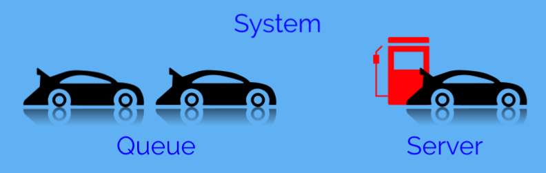
Consider the example of a petrol station (the system) which has only one fuel dispenser (the server). A car (a customer) arriving at the petrol station would join a queue and goes immediately to the fuel dispenser if no car is being served. Otherwise it would stay in the queue and wait to be served. So the petrol station (as the system) is made up of two components, namely the dispenser (as the server) and the queue. Thus the state of the system is described completely by the state of the server and the state of the queue. From knowing the state of the system, we can derive various results about the system that would be helpful for the business in order to be able to make changes to improve the quality of the service and/or increase profitability. Such results include the average time a car spends in the queue, the average queue length and the proportion of time the dispenser is idle.
How do we model such a system?
We define a variable for each component of the system to quantify its state. These variables are called state variables. Hence let Q be the length of the queue at a particular time. Q can take on values from 0,1,2,3,… Let S be the number of cars at the server at a particular time. S can take on values 0 or 1, where 0 means that the server is idle and 1 means that the server is busy.
An event is something that happens to the system which changes the state of the system. The three types of events in this example are: “arrival”, “begin service” and “end service” (or “departure”). An arrival is an event because it increases the queue length Q by 1. A “begin service” is an event since it decreases the queue length by 1 and increases S by 1 (S becomes equal to 1), since it takes a car from the queue and shifts to the server. An “end service” is an event because it decreases S by 1 (S becomes equal to 0).
An event calendar is a list of the types of events and their timings. This list is sorted in ascending form by time. The process of writing down an event on this calendar is called event scheduling. The computer goes through this list one-by-one and carries out each event. Thus each type of event has an associated event routine which tells the computer what to do to the system when executing that event. So the computer goes through the first row of the event calendar. The time of the system t (the time now) takes the time of this event and carries out its event routine.
The event routine for an “arrival” is made up of:
- schedule the next “arrival” event now (at time t) + inter-arrival time
- increase Q by 1
- if server is idle (S=0), then schedule “begin service” now (at time t).
The first point ensures that the system is maintained by an inflow of arriving cars. Hence you would always know when the next arrival will happen. The inter-arrival time which would be the time interval to the next event is usually generated randomly through an adequate probability distribution like the exponential distribution. The third point ensures that the server is never left empty when there are cars in the queue.
The event routine for a “begin service” is made up of:
- decrease Q by 1, increase S by 1
- schedule “end-service” at time t + service time.
Similarly the service time is usually generated from a suitable probability distribution like the exponential distribution.
The event routine for an “end service” is made up of:
- decrease S by 1
- if Q>=1, schedule “begin service” now (at time t).
Similar to the third point of the event routine of an “arrival”, this second point ensures that the server is never left empty when there are cars in the queue. When an event routine is carried out, the computer records the time (of the occurrence of the event) together with the values of the state values Q and S. The place where this data is stored is called the history. The computer then makes sure that the event calendar is sorted by time in ascending form, updates again the value of the time and executes the next scheduled event. This process is repeated over and over again until some specified condition closes the system, say for example, no more arrivals are allowed after 2 hours. On the other hand something must be done to open (initialise) the system. In order to open the system one must specify the initial time value t to be 0, and let the starting values of Q and S be 0. To start off the system one must schedule the first arrival at time 0 plus some inter-arrival time.
The code
Suppose that the system that we are modelling, has its inter-arrival time following an exponential distribution with mean 3 minutes and its service time following an exponential distribution with mean 2 minutes. We use the R software to model this system.
Inputs
The first part describes the input of the model. The lambda is the arrival rate which is 1/3 customers per minute. This is equivalent to the fact that the inter-arrival time has mean 3 minutes. The mu is the service rate which is 1/2 customers per minute. This is equivalent to saying that the mean service time is 2 minutes. The threshold is 120 minutes (2 hours), that is the system will not accept customers who arrive after 120 minutes. Hence at that time the system finishes off the customers already in the system and closes.
lambda<-1/3 #arrival rate
mu<-1/2 #servicing rate
threshold<-120
Initialisation
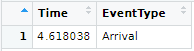
The initial time value t is set to 0. The initial queue length Q and the number of customers being served S are set to 0. That is, initially the system is empty. Then later on when the simulation starts, the values of Q and S change along the value of t. The code creates the event calendar, which is a data frame with its first column Time and its second column Event Type. In order to initialise the process, the code generate an exponential random variable with mean lambda, which is the time of the first arrival. This arrival is scheduled on the event calendar.
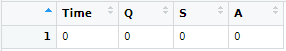
The code sets up the history of the simulation. This will keep track of all the data needed in order to extract results about the system when conducting the analysis after the simulation. Note that we have introduced another variable A, which will count the number of arrivals till time t. Initially, at time t is 0, A is set to 0. The variable A is only used for the history and thus at the end the simulation we will have note of how many customers have visited our system. The history is represented as a data frame storing the time and the state variables Q and S and the variable A. Prior to the start of the simulation, the history stores the initial values of t, Q, S and A.
set.seed(100) #ensure that you obtain the same simulation output each and every time

t<-0 #initial time value is 0
Q<-0 #initial queue length is 0
S<-0 #initial state of serve is 0 (idle)
A<-0 #total number of customers arriving at system till time t

Calendar<-data.frame(Time=double(),EventType=character(),stringsAsFactors = FALSE) #creating the event calendar
Calendar[nrow(Calendar)+1,]<-data.frame(t+rexp(1,lambda),"Arrival",stringsAsFactors = FALSE) #scheduling the first arrival

History<-data.frame(Time=double(),Q=double(),S=double(),A=double(),stringsAsFactors = FALSE) # creating a data frame with the history of the state values
History[nrow(History)+1,]<-data.frame(t,Q,S,A) #recording the initial time and state values

View(Calendar)
View(History)
The code produces the following initial event calendar and history.
Simulation
The code goes through the event calendar and reads the first row. The event calendar is sorted in ascending order by time and thus the first row is the next event that the code must carry out by executing its routine. The code updates the time with the time of this event currently taking place. Then it reads off the type of this events and carries out the routine associated with this event type. After the event routine is executed, the code stores the value of t, and the values of Q, S and A in the history, and thus captures the changes the event has done to the system. The code sorts the event calendar by time in ascending order and repeats the same thing over and over again, until there are no more events scheduled on the event notice. Note that the threshold is used so that the code accepts no more arrivals after a certain time unit. This ensure that the code reaches the point of having no events on the notice and thus forces the simulation to stop. Note also that when an arrival event is executed, the value of A is incremented by one because an arrival of a customer means that another customer has visited our system.
while(nrow(Calendar)>0)
{
t<-Calendar[1,1]
if(Calendar[1,2]=="Arrival"){
      a<-rexp(1,lambda)
      if(t+a<=threshold){Calendar[nrow(Calendar)+1,]<-data.frame(t+a,"Arrival",stringsAsFactors = FALSE)}
      Q<-Q+1
      A<-A+1
      if(S==0){Calendar[nrow(Calendar)+1,]<-data.frame(t,"BeginService",stringsAsFactors = FALSE)}
      }else{if(Calendar[1,2]=="BeginService"){
        Q<-Q-1
        S<-S+1
        Calendar[nrow(Calendar)+1,]<-data.frame(t+rexp(1,mu),"EndService",stringsAsFactors = FALSE)
      }else{
        S<-S-1
        if(Q>=1){Calendar[nrow(Calendar)+1,]<-data.frame(t,"BeginService",stringsAsFactors = FALSE)}
      }}
History[nrow(History)+1,]<-data.frame(t,Q,S,A)
Calendar<-Calendar[-1,]
Calendar <- Calendar[order(Calendar$Time),]
}

View(History)
The code produces the following history, which will be the data from which we can extract various results about our system.
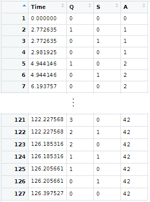
In the case of rows with the same value of t, we keep the row related to the event that was executed the most recently. For example row 2 of the history shown above represents the event when a car arrives at a station and row 3 represents the event when the car is shifted immediately to the idle dispenser. We keep row 3 and omit row 2. Also, we construct another variable N, the number of customers in the system, where N=Q+S.
#deleting the rows with duplicated time values, keeping the recent values of Q,S,A

RepeatedRows<-c()
for (i in 1:(nrow(History)-1))
if(History$Time[i]==History$Time[i+1]){RepeatedRows<-c(RepeatedRows,i)}
History<-History[-RepeatedRows,]

#adding column with total number of customers in the system, where N=Q+S

History$N<-History$Q+History$S 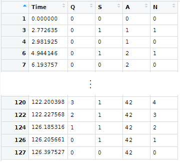
Results
The number of customer visiting the system during the simulation is 42 customers. The total time the simulation takes is 126.4 minutes. Note that the last arrival happened before the threshold (120 minutes), however the system needed more time to serve the remaining customers already in the system at that time.
TotalArrivals<-History$A[nrow(History)] #Total number of customers visiting the system
TotalArrivals

SimulationTime<-History$Time[nrow(History)] #Time from opening until max of threshold and time when last customer leaves system
SimulationTime
The following plot shows how the length of the queue changed over time during the simulation. Note that the queue length seems to oscillates between 0 and 2 before 95 minutes into the opening of the system. During this time, the queue is still picking up. This is known as the transient state of the system. Then the queue oscillates between 4 and 5 after 95 minutes and until the system closes (at time 120). Here the system is said to be in steady-state, that is, it reaches a more or less stable state. Hence the queue length oscillates between some close number and does not explode in size and thus destabilise the system.
plot(History$Time,History$Q,type="s",main="Queue Length",xlab="Time",ylab="Queue Length", yaxt="n")
axis(side = 2, at = seq(0,max(History$Q),1)) 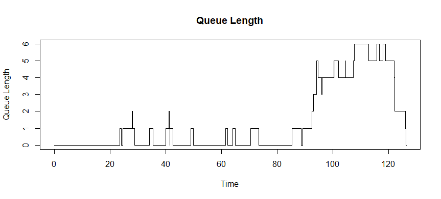
The next plot shows the time at which the server is busy (represented by 1) and when it is idle (represented by 0).
plot(History$Time,History$S,type="s",main="State of Server",xlab="Time",ylab="State", yaxt="n")
axis(side = 2, at = c(0,1)) 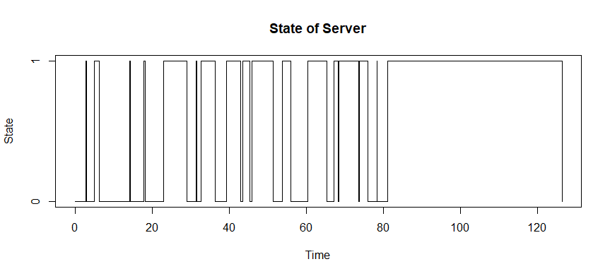
The following plot shows how many customers are present inside the system during the time of the simulation.
plot(History$Time,History$N,type="s",main="System Size",xlab="Time",ylab="System Size", yaxt="n")
axis(side = 2, at = seq(0,max(History$N),1)) 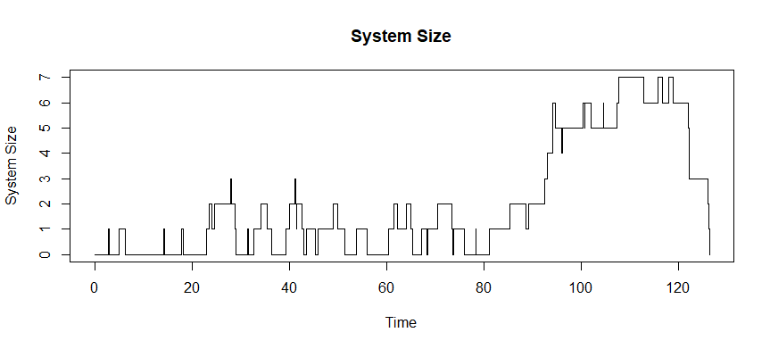
In order to obtain statistics on the queue of the system, we do some data wrangling on our history. We consider the intervals between the events listed in the history and the state of the queue during that time interval.
QueueData<-data.frame(LengthofTime=diff(History$Time,1),QueueLength=History$Q[-length(History$Q)])
View(QueueData) 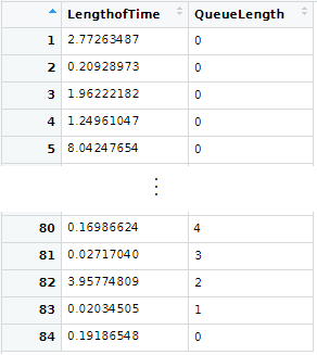
The collective total queue time is 169.5 minutes. So collectively the 42 customers spent 169.5 minutes in the queue. Thus the average time a customer spends in the queue is 4 minutes and the average queue length is 1.3 customers. Hence a customer entering the system should expect to see one or two customers in the queue.
TotalQueueingTime<-sum(QueueData$LengthofTime*QueueData$QueueLength)
TotalQueueingTime

AverageQueueLength<-TotalQueueingTime/SimulationTime
AverageQueueLength

AverageQueueingTime<-TotalQueueingTime/TotalArrivals
AverageQueueingTime
The following is some statistics about the server. The collective time spend by all the 42 customers at the server is 83.8 minutes. Thus the average time a customer spends being served is 2 minutes, which coincides with the fact that the service time follows an exponential distribution with mean 2 minutes (even though some variability might have been expected due to the simulation). The service utilisation is the proportion of time the server is busy. This is equal to 66.3 % in our simulation.
ServerData<-data.frame(LengthofTime=diff(History$Time,1),ServerUtilisation=History$S[-length(History$S)])
View(ServerData)

TotalServiceTime<-sum(ServerData$LengthofTime*ServerData$ServerUtilisation)
TotalServiceTime

ServerUtilisation<-TotalServiceTime/SimulationTime
ServerUtilisation

AverageServiceTime<-TotalServiceTime/TotalArrivals
AverageServiceTime
Similarly, one can obtain similar results on the number of customers at the system. The collective total time spent by the customers at the system is 253.3 minutes. Thus on average a customer spends 6 minutes at the system. Note that it was already noted that a customer expects to wait 4 minutes at the queue and spends on average 2 minutes at the server. The average system size is 2 customers. Hence a customer arriving at the system expects to see around 2 people already inside the system.
SystemData<-data.frame(LengthofTime=diff(History$Time,1),SystemSize=History$Q[-length(History$Q)]+History$S[-length(History$S)])
View(SystemData)

TotalTimeInSystem<-sum(SystemData$LengthofTime*SystemData$SystemSize)
TotalTimeInSystem

AverageSystemSize<-TotalTimeInSystem/SimulationTime
AverageSystemSize

AverageTimeInSystem<-TotalTimeInSystem/TotalArrivals
AverageTimeInSystem
Why do we use simulation and Next Event Simulation in particular?
In queueing theory, various models are studied from a mathematical perspective. For example, the example used here is called the M/M/1 model, where the first letter M (standing for Markovian) denotes that the inter-arrival time follows an exponential distribution, the second letter M denotes that the service time follows an exponential distribution and 1 denotes that there is just one server. The theory gives precise mathematical equations for the server utility (proportion of time the server is busy), the distribution of the number of people in the system and in the queue, and various other measures. In queueing theory various other equations are found for generalisations of such model like when there is more than 1 server or when the system has a limited capacity or when the service time distribution is general.
If the real-world system that needs to be modelled follows (more or less) one of these well-studied models, one should opt for the theoretical formulas in order to extract precise results about the system very quickly. On the other hand, in real-life scenarios, most systems have a nature that can differ widely from the well-studied models, and hence one should run on simulation on a model built in a way that mimics the real-world scenario really well. Possible deviations from the well-studied models are derived from situations like when the service times of different servers have different distributions, the average service times of different types of customers are different, the arrival rate changes with time, the inclusion of costs and penalties and much more.
In a dynamic model in which the state of the system does not change between the happening of an event and another, the code does not need to do any calculations to quantify the system state. In Next Event Simulation, the calculations are only done at the time points when the events happen. Thus this is more efficient (less time computational time needed) and accurate, than say calculating the system state at very small regular time intervals.