Generating Non Isomorphic Graphs in IGraph in R
Introduction
In this article we are going to show how to generate all the non-isomorphic graphs up to eleven vertices using the igraph package in R. In the Wolfram Mathematica software, one can find the function “ListGraphs[n]”, which output a list of all the non-isomorphic graphs on n vertices. However there seems to be no similar function in the igraph package in R. Here we will prove a procedure and code that gives us the adjacency matrix of each non-isomorphic graph up to eleven vertices.
The number of non-isomorphic graphs on n vertices
The table below shows the number of non-isomorphic graphs up to 11 vertices, as given by the On-Line Encyclopedia of Integer Sequences.
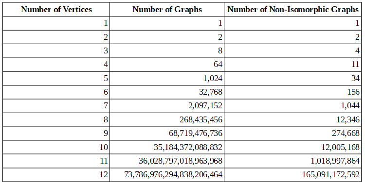
The number of non-isomorphic graphs grow exponentially with the number of vertices. Hence that is the reason why only graphs up to eleven vertices are considered.
A list of non-isomorphic graphs up to 11 vertices
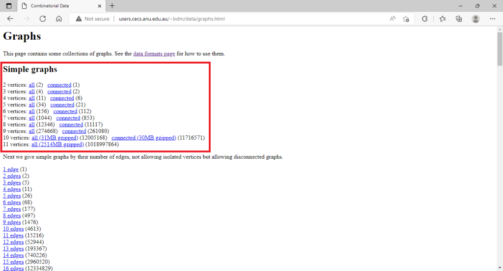
In his website (link available here), the mathematician Brendan McKay provides a list of all the non-isomorphic graphs up to 11 vertices in .g6 (or graph6) format. Go ahead and click the links on such a webpage to download such files. I used the files “all” which gives a list of all the graphs on n vertices, both connected and disconnect. However you could opt for the files “connected” which will give you the list of just the connected graphs on n vertices. Save the files as: “graph2.g6″,”graph3.g6″,…,”graph11.g6”.
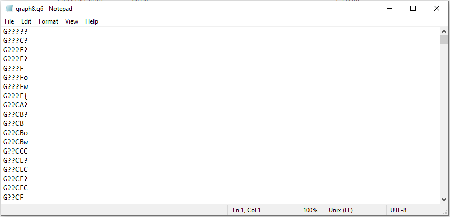
You can open your .g6 files with a text editor like Notepad. For example “graph8.g6” looks as follows. Each line, i.e, each code, represents one of the 12,346 non-isomorphic graphs on 8 vertices.
Decoding .g6 format
In his webpage (link available here) Brendan McKay describes how a graph is encoded into graph6 format. The reason for such encoding is obviously compactability. Here I will explain via an example how to decode the .g6 format to obtain the graph. Later on we will do this systematically on all the list, through a code in R.
Consider for example the code “G?`DDc” in graph6 format which is the 1000th graph in the list of non-isomorphic graphs in 8 vertices. The code is in ASCII characters which can be converted into a sequence of decimal numbers by using the conversion table like this.
Hence: “G?`DDc” becomes “71, 63, 96, 68, 68, 99”
Then we deduct 63 from each term of the sequence and obtain: 8, 0, 33, 5, 5, 36
The first term which is 8, describes the number of vertices in the graph and hence we note it and exclude it from the sequence.
The terms of 0, 33, 5, 5, 36 are converted into binary form of length 6.
Hence 0, 33, 5, 5, 36 becomes 000000 100001 000101 000101 100100
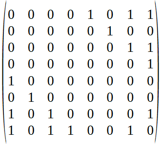
The next step is to draw an 8×8 adjacency matrix as follows:
Take the sequence 000000 100001 000101 000101 100100 from the left and fill up the matrix cells as indicated by the red arrow below:
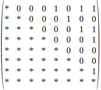
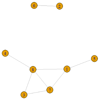
Finally replace the diagonal of the adjacency matrix by 0 and reflect the upper triangle into the lower triangle. The final adjacency matrix and its associated graph is shown below.
R code to convert graph6 format into adjacency matrices
The input of the following R code is .g6 file, for example let us consider “graph8.g6”, the list of all non-isomorphic graphs on 8 vertices. It is important for you to change the first line of code related to the working directory. Replace the input of setwd() with the path where you saved the file “graph8.g6”. This will be the same path where you will then find the output of the R code.
setwd("G:/*************")

## Data from  http://users.cecs.anu.edu.au/~bdm/data/graphs.html ##

Data<- read.delim("graph8.g6",header=FALSE)

DataFrame<-data.frame() #Creating empty data frame to store adjacency matrices

G<-as.character(Data[1,1])
n<-as.numeric(charToRaw(substr(G, 1, 1)))-63
n #number of vertices of the graph


for(k in 1:nrow(Data)){

  G<-as.character(Data[k,1])

vector<-c()
for(i in 2:nchar(G)){
vector<-c(vector,rev(as.numeric(intToBits(as.numeric(charToRaw(substr(G, i, i)))-63)[1:6])))}
vector

A<-matrix(0,nrow=n,ncol=n)
vector2<-vector
for(j in 2:n){
  for(i in 1:(j-1)){
    A[i,j]<-vector2[1];
    vector2<-vector2[-1]
  }}#filling the upper triangle of the adjacency matrix
for(i in 2:n){
  for(j in 1:(i-1)){
  A[i,j]<-A[j,i]
  }}#filling the lower triangle of the adjacency matrix
A

Avec<-as.vector(A)
DataFrame<-rbind(DataFrame,Avec)
if(k%%10000==0){print(k)}
}

colnames(DataFrame)<-NULL
write.csv(DataFrame,paste0("graphs",n,".csv"),row.names=FALSE)
This will output a csv file named “graphs8.csv” with a list of the adjacency matrices of all the non-isomorphic graphs on 8 vertices, which looks as follows:
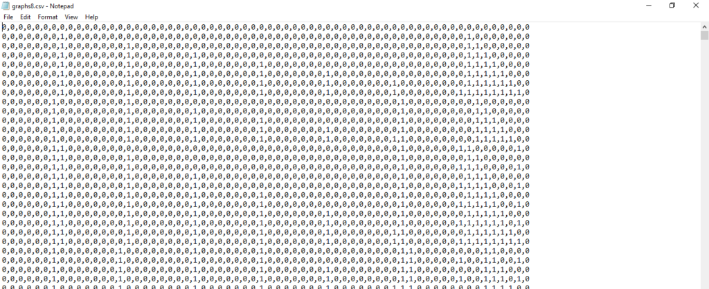
Each row correspond to an adjacency matrix to of one of the non-isomorphic graphs on 8 vertices. This could then be easy used with the function “graph_from_adjacency_matrix” of igraph in order to plot the graph from the adjacency matrix, which is given in the code below. Again change the working directory to the folder in which the files with the adjacency matrices are saved. The second line of code, shows that we are considering the non-isomorphic graphs on 8 vertices. The third line of code indicates that we are plotting the 1000th graph. Here you can change the number to any integer between 1 and 12,346.
setwd("G:********")

Data<- read.csv("graphs8.csv",header=FALSE,sep=",")

i<-1000 #graph number in list

library(igraph)
g<-graph_from_adjacency_matrix(matrix(as.vector(t(Data[i,])),nrow=sqrt(length(as.vector(t(Data[i,]))))),mode="undirected")
plot(g)
This piece of code will output the 1000th non-isomorphic graph on 8 vertices.