What is a threshold graph?

Introduction

Threshold graphs form a class of networks with a very elegant structure and can be depicted in layers of groups of vertices which are similar to each other. These graphs were first described by Chvatal and Hammer in 1977. Threshold graphs can be defined in a number of equivalent ways. Every definition will help us understand the structure of such graphs from a particular point of view. One of these definitions is used to construct and enumerate such graphs from a binary sequence and also leads us to test whether or not a given graph is a threshold graph.

We will provide custom R codes of functions, that test whether or not a graph is threshold, extract the compact creation sequence from the creation sequence, draw the layer-cake diagram of a threshold graph from its creation sequence, and plot the actual threshold graph from its creation sequence using the layout of the layer-cake diagram. We will be using the R package “igraph” which is specifically built for graph theory. This can be installed by using the command:

install.packages("igraph")

and loaded by the command:

library(igraph)

The R code for the functions used in this article can also be found on the github repository: MarkDebono/Threshold-Graphs-in-R (github.com)

Why is it called threshold graph?

Let’s start with the definition that gives this class of networks its name.

Definition 1: Let $G$ be a graph with vertex set $V(G)=\lbrace 1, 2,\cdots, n\rbrace$ and edge set $E(G)$ . The graph $G$ is a threshold graph if there exists a real number $S$ (called the “threshold value”) and a set of real-valued vertex weights $\lbrace w_1,w_2,\cdots,w_n\rbrace$ , such that $\lbrace i, j\rbrace\in E(G)$ if and only if $w_i+w_j>S$ .

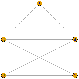
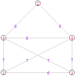
The following graph is displayed on the left is an example of a threshold graph on 5 vertices. In order to show that it is a threshold graph, we must find $S$ and a set of vertex weights that satisfy the condition given in Definition 1. Let the weights of the vertices be 3, 3, 4, 4, 5 respectively (as show in the graph displayed on the right) and let $S=5.5$ . We see that the sum of the weights of the two end-vertices of each edge is greater than 5.5. These are displayed as purple edge-weights on the graph on the right. There is no edge between vertex between 2 and 5, and between 1 and 5 because the sum of the weights of the end-vertices is $5 (<5.5=S)$ in both cases.

Now consider the following graph.

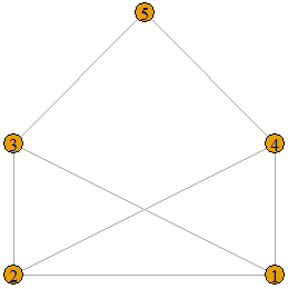
When one tries to find a set of vertex weights and a threshold value $S$ that separates the edges from the non-edges, it turns out to be a difficult task. This is not possible because the graph is not a threshold graph. However, in order to prove this fact, we must prove that no combination of weights and threshold value will satisfy Definition 1. Let us prove this by contradiction. Suppose there are weights $w_1, w_2, w_3,w_4,w_5$ and $S$ that satisfy Definition 1.

$\begin{equation*} \begin{split} & \lbrace 1, 5\rbrace\notin E(G)\mbox{ and }\lbrace 4, 5\rbrace\in E(G)\\ \Rightarrow & w_1+w_5 \leq S\mbox{ and }w_4+w_5 > S\\ \Rightarrow & w_4>w_1. \end{split} \end{equation*}$

On the other hand,

$\begin{equation*} \begin{split} & \lbrace 1, 3\rbrace \in E(G)\\ \Rightarrow & w_1+w_3 >S\\ \Rightarrow & w_4+w_3 >S \mbox{ (since }w_4 > w_1)\\ \end{split} \end{equation*}$

But $\lbrace 3,4\rbrace$ is not an edge of the graph. Hence this is a contradiction and thus we have shown that this is not a threshold graph.

The following equivalent definition describes how any threshold graph can be constructed from a single vertex through two graph operations.

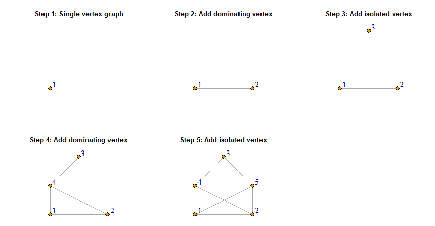
Definition 2: A threshold graph is a graph that is obtained from the single-vertex graph by repeated addition of an isolated vertex or a dominating vertex.

By adding a dominating vertex, we mean that we add a vertex to the graph and add edges from this vertex to any other vertex already present in the graph. As an example, let us construct a threshold graph on 5 vertices by starting from the single-vertex graph and adding a dominating vertex, an isolated vertex, a dominating vertex and another dominating vertex.

The creation sequence

Every threshold graph has a unique binary sequence that describes its construction.

Definition: The creation sequence of a threshold graph $G$ on $n$ vertices is a binary sequence $(c_2,c_3,\cdots, c_n)$ of length $n-1$ where $c_i=0$ shows that the $i^{th}$ vertex is added to the graph as an isolated vertex and $c_i=1$ shows that the $i^{th}$ vertex is added to the graph as a dominating vertex.

Various characteristics of threshold graphs can be deduced from this. First of all, a threshold graph is connected if $c_n=1$ and in this case, the threshold graph has at least one dominating vertex (i.e. a vertex connected to every other vertex in the graph). Thus a connected threshold graph has a creation sequence of the form $(c_2,c_3,\cdots,c_{n-1},1)$ and it can be shown that that there are $2^{n-1}$ non-isomorphic (distinct/different, ignoring vertex labelling) connected threshold graphs on $n$ vertices. If the restriction of connectedness is relaxed, then there are $2^n$ non-isomorphic threshold graphs on $n$ vertices.

The following R function named “GraphFromSeq”, draws a threshold graph from the creation sequence.

GraphFromSeq<-function(Seq){
  g<-graph.empty(1,directed="FALSE");
  for (i in 1:length(Seq)){
    g<-add.vertices(g,1);
    if(Seq[i]==1){for(i in 1:{vcount(g)-1}){g<-add.edges(g,c(i,vcount(g)))}}};
  plot(g)}

As an example, let us plot the threshold graph with creation sequence $(1,0,1,1)$ .

GraphFromSeq(c(1,0,1,1))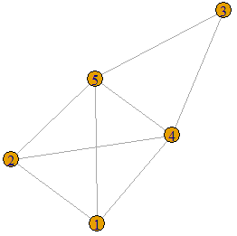

Testing whether or not a graph is a threshold graph

Suppose that we have a threshold graph. By Definition 2, we know that this graph is constructed from a single vertex by a sequence of additions of either isolated or dominating vertices. Now let us deconstruct the threshold graph back to the single-vertex graph. Let the vertices be labelled sequentially according the construction described in Definition 2. If the $n^{th}$ vertex is a dominating vertex (or equivalently the threshold graph is connected), remove it and all its incident edges. Otherwise, if the $n^{th}$ vertex is an isolated vertex, remove it. Either way, you end up with a threshold graph with $n-1$ vertices. The process of deleting the last vertex is repeated until the graph ends up as a single vertex. Now suppose that this process is carried on a graph which is not a threshold graph. There is a stage in the process in which the vertex with the highest degree is not a dominating vertex of the graph and the vertex with lowest degree is not an isolated vertex of the graph. The process to decompose the graph to a single-vertex is not possible. This is provides us with a test that determines whether or not a graph is threshold. The test is carried out by custom R function “is.threshold” which accepts a graph its input.

is.threshold<-function(g){
degseq<-degree(g,V(g))
degseq<-sort(degseq,decreasing=TRUE) #sorting the degree sequence in non-increasing form

repeat{
degseq<-degseq[degseq!=0];
if(length(degseq)==0){print("Graph is threshold");break};
if(degseq[1]==length(degseq)-1){degseq<-degseq[-1];degseq<-degseq-1}else{print("Graph is not threshold");break}}}

For example, let us construct a graph from an adjacency matrix and check whether or not it is a threshold graph.

A<-matrix(c(0,1,1,1,1,0,0,0,1,0,0,1,1,0,1,0),nrow = 4,ncol=4,byrow=TRUE)
g<-graph.adjacency(A,"undirected")
plot(g)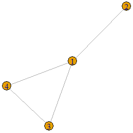

is.threshold(g)

Let us run the test on another graph.

A<-matrix(c(0,1,1,1,0,1,0,1,1,0,1,1,0,0,1,1,1,0,0,1,0,0,1,1,0),nrow = 5,ncol=5,byrow=TRUE)
g<-graph.adjacency(A,"undirected")
plot(g)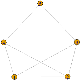

is.threshold(g)

The compact creation sequence

The creation sequence can be represented in compact form. Consider the creation sequence $(c_2,c_3,\cdots,c_n)$ . We classify a creation sequence into two types. When $c_2=0$ , we say that it is of type 0 and when $c_2=1$ , we say that it is of type 1. The compact creation sequence is created as follows. Let $a_1$ be the length of the first run of consecutive equal entries plus 1, let $a_2$ be the length of the second run of consecutive equal entries, let $a_3$ be the length of the third run of consecutive equal entries, and so on, up to the $k^{th}$ run. Then $(a_1,a_2,\cdots,a_k)$ (of type $c_2$ ) is the associated compact creation sequence.

The following R function, computes the compact creation sequence from the creation sequence.

CompSeq<-function(Seq)
{CompSeq<-c()
Counter<-1
CompSeq[Counter]<-2
Type<-Seq[1] #type of the 1st group
for(i in 2:length(Seq))
{if(Seq[i]==Seq[i-1]){CompSeq[Counter]<-CompSeq[Counter]+1}else{Counter<-Counter+1;CompSeq[Counter]=1}};
return(list(Sequence=CompSeq,Type=Type))}

We give two examples.

CompSeq(c(0,0,0,1,1,1,0,0,0,0,1,1,1,1,0,1))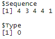

CompSeq(c(1,0,0,0,1,1,1,1,0,0,0,1,1,1,0))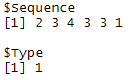

The Layer-Cake Diagram

We use the compact creation sequence to draw a representation of the structure of a threshold graph known as the layer-cake diagram. This diagram has two columns and different layers. Consider the compact creation sequence $(a_1,a_2,\cdots,a_k)$ of type 0 for the time being. The set $A_1$ (of vertices) of size $a_1$ is drawn on the left of layer 0 (the bottom layer) and the set $A_2$ of size $a_2$ is drawn on the right of layer 0. The set $A_3$ of size $a_3$ is drawn on the left of layer 1 (the layer above layer 0) and the set $A_4$ of size $a_4$ is drawn on the right of layer 1. This process is continued until all the $k$ sets are drawn. The sets drawn on the left of the layer-cake diagram are called “isolating sets” and the sets drawn on the right are called “dominating sets”. There is an edge between a dominating set and every other dominating set, and a dominating set and the isolated sets on its layer or below. An isolating set $A_i$ represents an empty induced subgraph on $a_i$ vertices of the threshold graph and a dominating set $A_i$ represents a complete induced subgraph on $a_i$ vertices of the threshold graph. An edge between the sets $A_i$ and $A_j$ in the layer-cake diagram represents the presence of edges between every vertex in $A_i$ to every vertex in $A_j$ .

The following R function named “LayerCake” draws the layer-cake diagram of a threshold graph, directly from its creation sequence. Note that it makes use of the function “ComSeq”.

LayerCake<-function(Seq){
  if(CompSeq(Seq)$Type==0){CakeSeq<-rep(c(1,0),length.out=length(CompSeq(Seq)$Sequence)-1)}else{CakeSeq<-rep(c(0,1),length.out=length(CompSeq(Seq)$Sequence)-1)}

g<-graph.empty(1,directed="FALSE")
for (i in 1:length(CakeSeq)){g<-add.vertices(g,1);if(CakeSeq[i]==1){for(i in 1:{vcount(g)-1}){g<-add.edges(g,c(i,vcount(g)))}}}
n<-vcount(g) #number of sets

if(CompSeq(Seq)$Type==0){
  l<-matrix(c(rep(c(-1,1),length.out=n),floor(seq(0,n,by=0.5))[1:n]),nrow=n,ncol=2,byrow=FALSE)
    if(n>=6)
  {curvededges<-c()
  for (i in seq(2,n-4,2))
  {for(j in seq(4+i,n,2))
  {curvededges<-c(curvededges,which(E(g)==E(g)[i %--% j]))}}
  E(g)$curved<-rep(0,ecount(g))
  E(g)$curved[curvededges]<--0.3}}else{
    l<-matrix(c(rep(c(1,-1),length.out=n),ceiling(seq(0,n,by=0.5))[1:n]),nrow=n,ncol=2,byrow=FALSE)
    if(n>=5)
  {curvededges<-c()
  for (i in seq(1,n-4,2))
  {for(j in seq(4+i,n,2))
  {curvededges<-c(curvededges,which(E(g)==E(g)[i %--% j]))}}
  E(g)$curved<-rep(0,ecount(g))
  E(g)$curved[curvededges]<--0.3}}

plot(g,layout=l,main="Layer-Cake Diagram",vertex.label=CompSeq(Seq)$Sequence)}

Consider the following example.

LayerCake(c(0,0,0,1,1,1,0,0,0,0,1,1,1,1,0,1))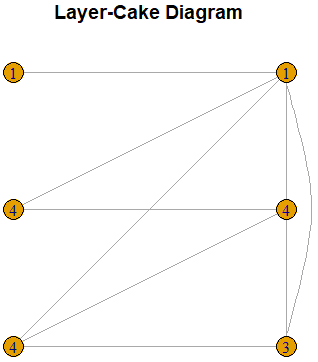

The construction of the layer-cake diagram when the type of sequence is 1 (that is, the first set is a dominating set), is similar. In this case, the set $A_1$ is drawn on the right column of layer 0. The set $A_2$ is then drawn on the left column of layer 1, and so on. Hence, in this case layer 0 has just one set, the dominating set $A_1$ . The following is another example of a layer cake diagram.

LayerCake(c(1,0,0,0,1,1,1,0,0,0,0,1,1,1,1,0))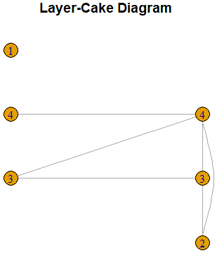

Recall that the layer-cake diagram is just a representation of the threshold graph, which helps us visualise and summarise the structure of the threshold graph. The next function named “ThresholdGraph” plots the actual threshold graph from the creation sequence using the layout of the layer-cake diagram. This function makes use of the previously defined function “CompSeq”.

ThresholdGraph<-function(Seq){
n<-length(CompSeq(Seq)$Sequence)

if(CompSeq(Seq)$Type==0){
  l<-matrix(c(rep(c(-1,1),length.out=n),floor(seq(0,n,by=0.5))[1:n]),nrow=n,ncol=2,byrow=FALSE)}else{
    l<-matrix(c(rep(c(1,-1),length.out=n),ceiling(seq(0,n,by=0.5))[1:n]),nrow=n,ncol=2,byrow=FALSE)}

l2<-c()
for(i in 1:length(CompSeq(Seq)$Sequence))
{if(CompSeq(Seq)$Sequence[i]==1){l2<-rbind(l2,l[i,])}else{rand<-runif(1,0,2*pi);
  l2<-rbind(l2,cbind(l[i,1]+0.1*cos(rand+2*pi/CompSeq(Seq)$Sequence[i]*seq(0,CompSeq(Seq)$Sequence[i]-1)),l[i,2]+0.1*sin(rand+2*pi/CompSeq(Seq)$Sequence[i]*seq(0,CompSeq(Seq)$Sequence[i]-1))))}
}

g<-graph.empty(1,directed="FALSE")
for (i in 1:length(Seq)){g<-add.vertices(g,1);if(Seq[i]==1){for(i in 1:{vcount(g)-1}){g<-add.edges(g,c(i,vcount(g)))}}}
plot(g,layout=l2,vertex.label=NA,vertex.size=6)}

ThresholdGraph(c(0,0,0,1,1,1,0,0,0,0,1,1,1,1,0,1))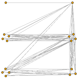

ThresholdGraph(c(1,0,0,0,1,1,1,0,0,0,0,1,1,1,1,0))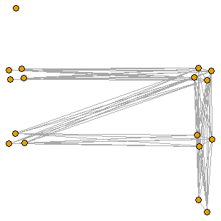

Conclusion

We have obtained some insight on the structure of threshold graphs from two equivalent definitions. One such definition provides us with a way of constructing threshold graphs and represent them by a unique binary sequence. From such a sequence, we can easily enumerate the number of non-isomorphic threshold graphs on a given number of vertices. Moreover we use R to depict the layer-cake diagram of a threshold graph and also the actual graph in the layout of its layer-cake diagram.