How to calculate core deposits

Introduction & Definition of Core Deposits

Lending banks use their deposits as one of the main sources of funding . In order to mitigate risk of capital inadequacy and liquidity risk, it is important for the bank to partition the deposits’ balance into two parts: the core deposits (a.k.a. sticky deposits) and the non-core deposits (a.k.a. non-sticky deposits). Core deposits are loosely defined as deposits that form a stable source of funds for lending.

In the case of term deposits, depositors lend a sum of money to the bank and cannot withdraw it before a stipulated date known as the maturity date. Hence the bank would be certain that such an amount will remain as part of the deposits till that particular maturity date. By doing some workings, the bank can easily calculate how much of the deposits (at the current date) will stay in the bank for a further 1 year, 2 years, 3 years, etc…

On the other hand, non-term deposits have no maturity date, and the depositors can withdraw their money at any time and at whatever the amount. A question that naturally arises is: how are we going to calculate the stability of non-term deposits given there is no restriction on the time when the depositor can withdraw the deposits and on the amount that could be withdrawn? We will thus define stability for non-term deposits in relation to time and with reference to probability.

Definition: The $\alpha$ % $t$ -time unit core deposits amount is the deposit amount that will stay in the bank for a further $t$ time units or more, with a probability of $\alpha$ %.

We can also define core deposits as a percentage.

Definition: The $\alpha$ % $t$ -time unit core deposits percentage is deposit amount that will stay in the bank for a further $t$ time units or more, with a probability of $\alpha$ %, divided by the total sum of deposits.

As an example, suppose that we currently have a balance of €100,000 non-term deposits. Suppose that we expect that at least €70,000 of such deposits will remain in the bank in 1-years’ time, with a probability of 90%. So, the 90% 1-year core deposits amount is €70,000 whereas the 90% 1-year core deposits percentage is $\frac{70,000}{10,0000}=70$ %.

We will calculate the core deposits for non-term deposits as follows.

Calculation of Core Deposits

Suppose that we have $n$ depositor accounts, and we collect their end-of-month balance for some period of time $T$ , for example, 2 years ( $T=24$ months), 5 years ( $T=60$ months) or 10 years ( $T=120$ months). The length of such a period of time should as long as the available data permits, given that all of it describes the current economic scenario. Let $X_{ij}$ be the end-of-month balance for depositor $i$ for month $j$ . Hence for depositor $i$ , we have the following time series of balances:

$\begin{equation*} X_{i1},X_{i2},\cdots,X_{iT} \end{equation*}$

We take the first difference of this series to obtain the monthly changes in the end-of-month balances for depositor $i$ :

$\begin{equation*} X_{i2}-X_{i1},X_{i3}-X_{i2},\cdots,X_{iT}-X_{i,T-1} \end{equation*}$

Let us relabel such a series as:

$\begin{equation*} Y_{i1},Y_{i2},\cdots,Y_{i, T-1}\mbox{ where }Y_{ij}=X_{i, j+1}-X_{ij} \end{equation*}$

Let us consider the 1-month ahead change $Y_{i,T}$ in the balance of depositor $i$ . We assume that this follows the discrete uniform distribution on the range $Y_{i1},Y_{i2},\cdots,Y_{i, T-1}$ . Now let us consider the 2-month ahead change $Y_{i,T}+Y_{i,T+1}$ in the balance of deposits $i$ . We assume that this is sum of two independent discrete uniformly distributed random variables each having a range $Y_{i1},Y_{i2},\cdots,Y_{i, T-1}$ . This pattern is carried on, until we obtain the distribution of all the monthly changes for a required future horizon.

The 1-month ahead change in the total deposits is given by: $Y_{1,T}+Y_{2,T}+\cdots + Y_{n,T}$ , where $n$ is the total number of depositors. This is actually the sum of $n$ discrete uniformly distributed random variable have a distinct range as stated above. The 2-month ahead change in the total deposits is given by: $Y_{1,T}+Y_{2,T}+\cdots + Y_{n,T}+Y_{1,T+1}+Y_{2,T+1}+\cdots + Y_{n,T+1}$ , and so on. It follows that for some positive integer $k$ , the $k$ -month ahead total deposits balance is equal to:

$\begin{equation*} \sum_{i=1}^{n} X_{iT}+\sum_{j=1}^{k} Y_{1,T+j-1}+\sum_{j=1}^{k} Y_{2,T+j-1}+\cdots + \sum_{j=1}^{k} Y_{n,T+j-1} \end{equation*}$

We will use simulation techniques in order to simulate the distributions of the $k$ -month ahead total deposits balances, from which we will derive the core deposits as their percentiles. Let us start with the distribution of the 1-month ahead change in the total deposits is given by: $Y_{1,T}+Y_{2,T}+\cdots + Y_{n,T}$ . Recall that the distribution of each $Y_{i,T}$ is discrete uniformly distribution on the range $Y_{i,1},Y_{i,2},\cdots,Y_{i,T-1}$ , for $i \in\lbrace 1,2, \cdots, n\rbrace$ . Hence the sequence $Y_{i,1},Y_{i,2},\cdots,Y_{i,T-1}$ can be taken as the empirical distribution of $Y_{i,T}$ . However for a more stable simulation we will use the sequence:

$\begin{equation*} Y_{i,1},\cdots,Y_{i,1}, Y_{i,2},\cdots,Y_{i,2}\cdots,Y_{i,T-1}\cdots Y_{i,T-1} \end{equation*}$

as the empirical distribution of $Y_{i,T}$ .

We derive the empirical distribution of the 1-month ahead balance for customer $i$ , namely $X_{iT}+Y_{i,T}$ , by computing:

$\begin{equation*} X_{iT}+Y_{i,1},\cdots,X_{iT}+Y_{i,1}, X_{iT}+Y_{i,2},\cdots,X_{iT}+Y_{i,2}\cdots,X_{iT}+Y_{i,T-1}\cdots X_{iT}+Y_{i,T-1} \end{equation}$

and replace the negative numbers by 0, because we assume that the deposit accounts can never have a negative balance.

We estimate the distribution of the 1-month ahead total balance $\sum_{i=1}^{n} X_{iT}+Y_{1,T}+Y_{2,T}+\cdots + Y_{n,T}$ from the distributions of $X_{iT}+Y_{i,T}$ (for all $i\in\lbrace 1,2,\cdots, n \rbrace$ ) by using Latin Hypercube Sampling as follows. Consider a random permutation of each empirical distribution of the random variable $X_{iT}+Y_{i,T}$ for all $i\in\lbrace 1,2,\cdots, n \rbrace$ . By adding these $n$ permutations component-wise, we obtain the empirical distribution of the 1-month ahead total balance. The $\alpha$ % 1-month core deposits amount is equal to the $(1-\alpha)^{th}$ percentile of this empirical distribution.

Next we estimate the distribution of the 2-month ahead total balance $\sum_{i=1}^{n} X_{iT}+\sum_{j=1}^{2} Y_{1,T+j-1}+\sum_{j=1}^{2} Y_{2,T+j-1}+\cdots + \sum_{j=1}^{2} Y_{n,T+j-1}$ . First let us consider each customer one-by-one. We have already obtained the empirical distribution of the 1-month ahead balance for customer $i$ denoted by the random variable $X_{iT}+Y_{i,T}$ . By using Latin Hypercube Sampling again, we add (component-wise) a permutation of the empirical distribution of $Y_{i,T}$ to the empirical distribution of $X_{iT}+Y_{i,T}$ . Then we replace the negative numbers by 0 and this will result in the empirical distribution of the 2-month ahead balance for customer $i$ . By summing (the permutations of ) the empirical distributions of each customer will result in the distribution of the 2-month ahead total balance. Its $(1-\alpha)^{th}$ percentile will represent the $\alpha$ % 1-month core deposits amount. Such method is extended to obtain the $\alpha$ % 3-month, 4-month etc… core deposits amounts.

This whole process of finding the core deposits for different time periods is repeated a number time, and the presented core deposits figures are the averages obtained from all the simulations. This will help the model to converge and present stable results.

Worked Example

The following is an example of the calculation of the core deposits on a portfolio of just 6 deposit accounts. However the simulation can be extended to much larger number of accounts, possibly hundreds of thousands. The csv file “Data.csv” together with all the R codes are available on my GitHub https://github.com/MarkDebono/Core-Deposits

Note that the working directory must be set to the folder in which the data file is stored. The data contains a series of 24 monthly balances for 6 customers, where each column is associated with a customer.

setwd("C:/Users/Deposits") #change this to the folder that contains the csv file "Data.csv"
Deposits<-read.csv("Data.csv",sep=",",header=TRUE)
head(Deposits)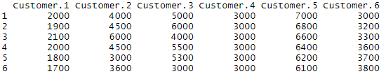

Deposits Data

tail(Deposits)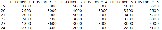

Deposits Data

Each of the 6 series is plotted in a grid of plot. The first three series are very typical. There are accounts whose balances display increases and decreases from one month to the other which look quite random. The last three series are the extreme cases. The balance in the account of customer 4 remains constant, the balance in the account of customer 5 is decreasing, whereas the balance in the account of customer 6 is increasing. Since we use the historic data to simulate the future account balance, the forecasted balances of customer 4, will always be 3000, the forecasted balances of customer 5 will be lower that its current balance of 2800 whereas the forecasted balances of customer 6 will be higher than its current balance of 7100. This will result into treating all of the current balances of customers 4 and 6 as stable, whereas a relatively low proportion of the current balance of customer 5 will be treated as stable (depending on the forecasting period).

library(ggplot2)
library(gridExtra)

gglist<-list()
for(i in 1:ncol(Deposits))
{gglist[[i]]<-local({i<-i;ggplot(Deposits,aes(x=seq(1:nrow(Deposits)),y=Deposits[,i]))+geom_line()+xlab("Month")+ylab("Amount")+ggtitle(paste("Customer",i))})}
grid.arrange(grobs=gglist, nrow = 2,ncol=3)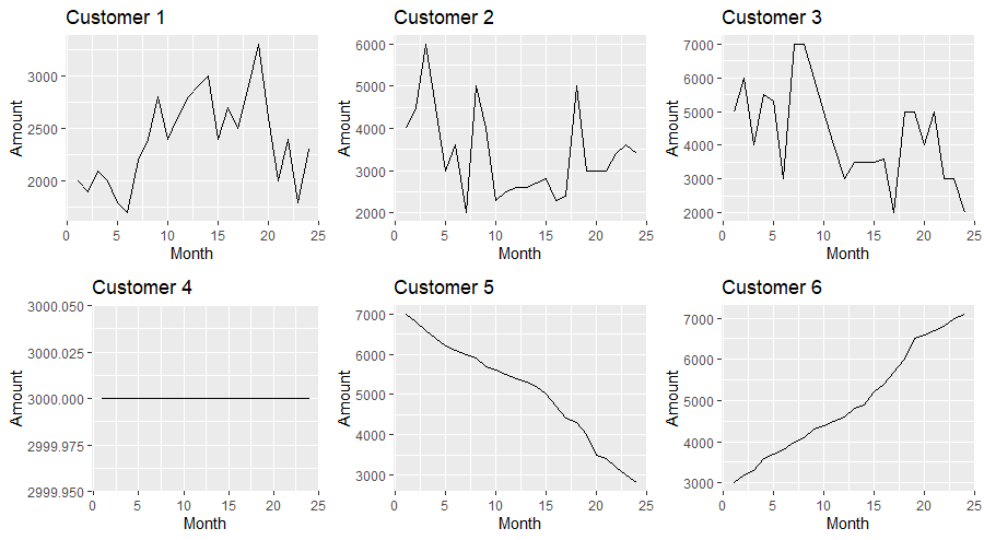

Deposits Plots

Next we perform the first differencing for all the 6 series (i.e. we obtain the monthly changes). These will be used in the simulation to forecast future balances.

DepDiff<-apply(Deposits,2,diff)
head(DepDiff)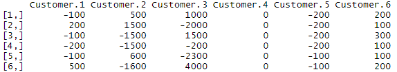

Changes in Balances

The variables “alpha”, “k” and “iter_no” are used in the simulation. The variable “alpha” represent the level of significance and here we are going to use alpha=0.95 in order to obtain the 95% core deposits. The variable “k” represents the length of the forecasting period. When we let k to be equal to 24, we will able to find the 95% core deposits amount for a period of 1 month, 2 months, 3 months, up to, 24 months. We will use the variable “iter_no” because the process of calculating the 95% core deposits amounts is repeated for a number of times, and the results are averaged out in order to ensure a stable output from the simulation. The variable “iter_no” is equal to the number of such repetitions. In this case “iter_no” is taken to be 100.

alpha<-0.95 #the level of significance associated with the core deposits
k<-24 #the number of months ahead for which we calculate the core deposits
iter_no<-100 #the number of iterations used

The following is the code for the simulation.

CoreDepositsAveraged<-rep(0,k)

for(iter in 1:iter_no)

{  
SimData<-Deposits[rep(nrow(Deposits),nrow(DepDiff)*4),]
rownames(SimData) <- 1:nrow(SimData)
SimData

CoreDeposits<-c()

for(m in 1:k)
{
for(i in 1:ncol(SimData))
{SimData[,i]<-SimData[,i]+sample(rep(DepDiff[,i],4))}
SimData[SimData<0]<-0 #Removing the negative balances

SimDataDash<-SimData
for(i in 1:ncol(SimDataDash))
{SimDataDash[,i][SimDataDash[,i]>Deposits[nrow(Deposits),][[i]]]<-Deposits[nrow(Deposits),][[i]]}

CoreDeposits<-c(CoreDeposits,quantile(rowSums(SimDataDash),1-alpha))
}
CoreDepositsAveraged<-(CoreDepositsAveraged*(iter-1)+CoreDeposits)/iter
}

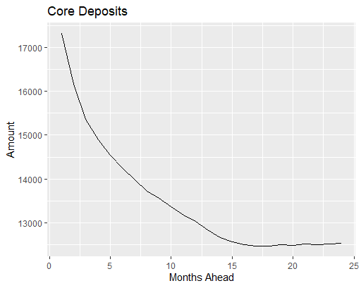
The following is the output from the simulation. The 95% core deposits amounts for a certain number of months ahead are shown in a table and in a plot.

Results<-data.frame(Months.Ahead = seq(1,k),Core.Deposits=CoreDepositsAveraged)
Results
ggplot(Results,aes(x=Months.Ahead,y=Core.Deposits))+geom_line()+xlab("Months Ahead")+ylab("Amount")+ggtitle("Core Deposits")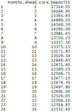

Core Deposits

Core Deposits Plot

We will make an amendment to ensure that the core deposits amounts are non-increasing with the time units. For example, if the 95% 20-month core deposits amount is 12491 we expect that the 95% 21-month, 22-month, 23-month and 24-month core deposits amounts are all less than or equal to 12491.

for(i in 2:nrow(Results))
{if(ResultsCore.Deposits[[i-1]]){ResultsCore.Deposits[[i-1]]}}

Results
ggplot(Results,aes(x=Months.Ahead,y=Core.Deposits))+geom_line()+xlab("Months Ahead")+ylab("Amount")+ggtitle("Core Deposits")

Core Deposits 2

Core Deposits Plot 2

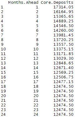
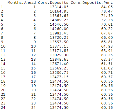
By dividing the core deposits amounts by the current total balance of the deposits, we can obtain the core deposits percentages. These are shown the table and plot below. For example we obtain a 95% 12-month core deposits percentage of 63.25%, that is, we expect that 63.25% of the current total deposits amount will remain in the accounts for a period of at least 12 months.

ResultsCore.Deposits*100/rowSums(Deposits[nrow(Deposits),]),2)
Results
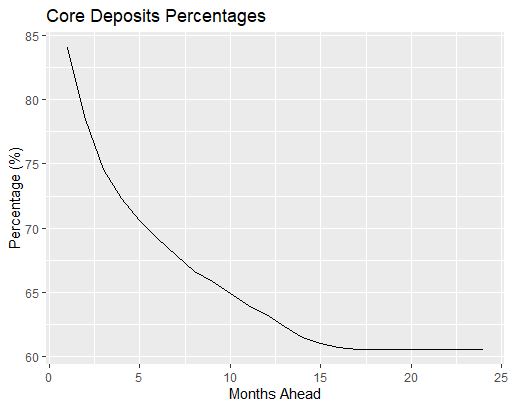
ggplot(Results,aes(x=Months.Ahead,y=Core.Deposits.Perc))+geom_line()+xlab("Months Ahead")+ylab("Percentage (%)")+ggtitle("Core Deposits Percentage")

Core Deposits Percentages

Core Deposits Percentage Plot