The Effect of Loan Prepayment on THe Balance Sheet
Introduction
We study the various effects of prepayment on a loan arising from two scenarios. We consider loans that are repaid by a sequence of fixed monthly instalments over a pre-stated number of months. The first scenario is that when the monthly repayment amount is increase by some fixed factor from some month onwards. The second scenario is that when there is a decrease in the interest rate during the lifetime of the loan, whilst the repayment amount is kept constant instead of revised downwards.
We define the prepayment rate based on the expected and the actual monthly outstanding principal, and in both instances we provide closed formulae for the actual duration of the loan and the monthly prepayment rate for each month, in terms of the loan parameters. Moreover we consider the interest income lost at each month due to the underlying prepayment.
The theory is extended to analyse the effects of prepayment on a portfolio of loans. The portfolio prepayment rate is computed together with the actual outstanding combined portfolio principal. This is an exercise for the asset-liability management of the lending institution. Together with the analysis of the future actual portfolio interest income inflow, all of this could be useful in the risk assessment of the loan portfolio.
The structure of the document is as follows. First we consider the repayment schedule of a loan, which provides the repayment structure of the loan given that prepayment is not present. Then scenario one in presented. We consider the case when prepayment starts immediately from the first month. Then this is extended to the general case in which the prepayment can start at any predetermined month. Finally the theory is extended to analyse a portfolio of loans. The second scenario is presented in a similar fashion.
The Repayment Schedule
Consider a loan which has an associated principal amount  , yearly interest rate
  compounded monthly and term
  months. The borrower pays back equal monthly payments of amount
  each, in order to redeem the loan. In fact, the repayment schedule which includes each monthly repayment broken down into the interest and capital component, and the monthly outstanding principal, can be computed from just the knowledge of , and . In other words , and define such a loan completely.
The repayment amount can be calculated from , and by using the equation:
(1) 
This follows from the fact that is the present value of payments each of amount each, using a discounting rate of  . It can be shown by induction that the interest component, the capital component and outstanding principal at month
  can be described in terms of , , and as follows:
Lemma 1: Consider a loan with associated principal , yearly interest rate compounded monthly and duration months. Let be the monthly repayment as calculated in equation (1). The interest and capital component in the  repayment and the outstanding principal at month , for
  , are given by:

From Lemma 1 we can obtain the proportion of the payment that corresponds to interest payment and the proportion that corresponds to the repayment of capital. These are obtained by the dividing the formulae for  and
and  by .
by .
Lemma 2: The proportions of the interest and capital component in the repayment for , are given by:

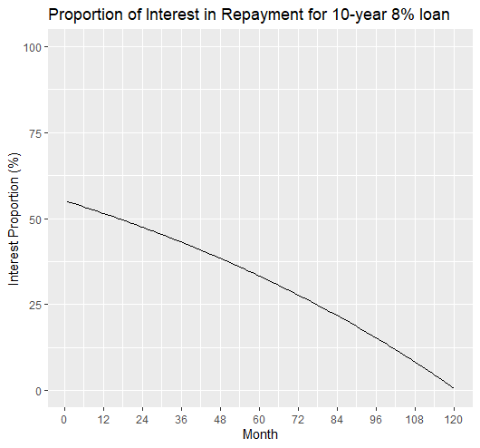
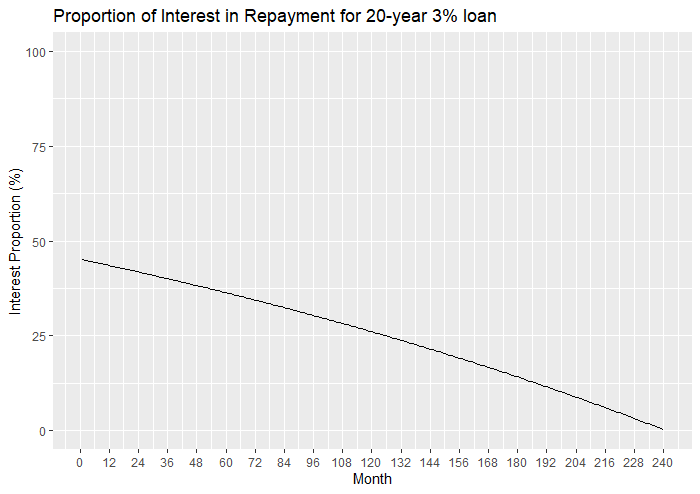
We see that these proportions do not depend on the loan principal . These depend on the term of the loan and the interest rate, and the payment number of the loan. The following two plots show the proportion of interest in the repayments over the life of a loan. We consider two examples. The first one is a 10-year loan ( ) with an interest rate of 8% and the second one is a 20-year loan (
 ) with an interest rate of 3%. Note that these plots also show the proportion of capital in the repayments, because
  for all . Thus we can see the decrease (or increase respectively) of the interest proportion (or capital proportion) with .
The sum of the capital components of all the repayments is equal to , the loan principal. The total interest paid on the loan is:

The proportion of the total interest paid over the Principal amount is independent of and depends only on and .

Constant Prepayment from Month 1
There are instances in which the borrower makes one or more monthly repayments that are greater than the value as determined by the repayment schedule. This results in what is known prepayment or early repayment of a loan. The prepayment rate of a loan at month is defined as the extra capital repaid until month divided by the outstanding principal according to the repayment schedule at month . This is given by the equation:
(2) 
where ,  stands for the outstanding principal according to the repayment schedule at month and
  stands for the actual outstanding principal at month .
Suppose we have a loan in which the borrower increases each monthly repayment by a factor of  , that is, each repayment is
  instead of the value as stated by the repayment schedule. We are after: (1) the prepayment rate at each month (2) the actual duration of the loan. First, from Lemma 1 we can deduce the capital, interest component and outstanding principal in this instance.
Lemma 3: Consider a loan with associated principal , yearly interest rate compounded monthly and duration months. Let be the actual repayment amount where the value as calculated in equation (1). Let  be the actual duration of the loan, given that prepayment is present. The interest and capital component in the repayment and the outstanding principal at month , for
  are given by:

Proof: By induction on . 
Result 1: Consider a loan with associated principal , yearly interest rate compounded monthly and duration months. When the actual monthly repayment is increased by a factor of , the prepayment rate at month , for  , is:
, is:
![\begin{equation*}\textup{Prepayment Rate}(k)=\frac{r[(1+\frac{i}{12})^k-1]}{1-(1+\frac{i}{12})^{k-n}}.\end{equation*}](https://datasciencegenie.com/wp-content/ql-cache/quicklatex.com-35ac676598dbd1b10d9261490e3266e9_l3.png "Rendered by QuickLaTeX.com")
Proof:
![\begin{equation*}\begin{split}\text{Prepayment Rate}(k)&= \frac{\text{Principal}_{\text{RS}}(k)-\text{Principal}_{\text{Actual}}(k)}{\text{Principal}_{\text{RS}}(k)} \text{ (by Equation 2})\\&=\frac{P(1+\frac{i}{12})^k-\frac{R(1+\frac{i}{12})^k}{(\frac{i}{12})}+\frac{R}{(\frac{i}{12})}-P(1+\frac{i}{12})^k+\frac{(1+r)R(1+\frac{i}{12})^k}{(\frac{i}{12})}-\frac{(1+r)R}{(\frac{i}{12})}}{P(1+\frac{i}{12})^k-\frac{R(1+\frac{i}{12})^k}{(\frac{i}{12})}+\frac{R}{(\frac{i}{12})}}\text{ (by Lemma 1(c)and Lemma 3(c))}\\&=\frac{\frac{rR(1+\frac{i}{12})^k}{(\frac{i}{12})}-\frac{rR}{(\frac{i}{12})}}{P(1+\frac{i}{12})^k-\frac{R(1+\frac{i}{12})^k}{(\frac{i}{12})}+\frac{R}{(\frac{i}{12})}}\\&=\frac{\frac{rR(1+\frac{i}{12})^k}{(\frac{i}{12})}-\frac{rR}{(\frac{i}{12})}}{\frac{R}{(\frac{i}{12})}(1-(1+\frac{i}{12})^{-n})(1+\frac{i}{12})^k-\frac{R(1+\frac{i}{12})^k}{(\frac{i}{12})}+\frac{R}{(\frac{i}{12})}} \text{ (by Equation 1})\\&=\frac{r(1+\frac{i}{12})^k-r}{(1-(1+\frac{i}{12})^{-n})(1+\frac{i}{12})^k-(1+\frac{i}{12})^k+1}\\&=\frac{r[(1+\frac{i}{12})^k-1]}{1-(1+\frac{i}{12})^{k-n}}.\mbox{ } \square\end{split}\end{equation*}](https://datasciencegenie.com/wp-content/ql-cache/quicklatex.com-f5a5cca504bdb6ffeeb5334e735117da_l3.png "Rendered by QuickLaTeX.com")
Result 2: Consider a loan with associated principal , yearly interest rate compounded monthly and duration months. When the actual monthly repayment is increased by a factor of , the actual duration of the loan is:
![\begin{equation*}\lceil \frac{\ln{(1+r)}-\ln{[r+(1+\frac{i}{12})^{-n}]}}{\ln{(1+\frac{i}{12})}} \rceil\end{equation*}](https://datasciencegenie.com/wp-content/ql-cache/quicklatex.com-c2a3b40439870cbbbd3dc1b6862c1080_l3.png "Rendered by QuickLaTeX.com")
Proof: Let be the least integer such that the prepayment rate is greater or equal to 1. Then is the actual duration of the loan. Note that we assume that  and hence
  .
.
![\begin{equation*}\begin{split}\text{Prepayment Rate}(k)&\geq 1\\\frac{r[(1+\frac{i}{12})^k-1]}{1-(1+\frac{i}{12})^{k-n}} &\geq 1\text{ (by Result 1})\\r(1+\frac{i}{12})^k-r &\geq 1-(1+\frac{i}{12})^{k-n}\\r(1+\frac{i}{12})^k+(1+\frac{i}{12})^{k-n} &\geq 1+r\\(1+\frac{i}{12})^k[r+(1+\frac{i}{12})^{-n}] &\geq 1+r\\(1+\frac{i}{12})^k&\geq\frac{1+r}{r+(1+\frac{i}{12})^{-n}}\\\ln{(1+\frac{i}{12})^k}&\geq \ln{\frac{1+r}{r+(1+\frac{i}{12})^{-n}}}\\k&\geq \frac{\ln{(1+r)}-\ln{(r+(1+\frac{i}{12})^{-n})}}{\ln{(1+\frac{i}{12})}}.\end{split}\end{equation*}](https://datasciencegenie.com/wp-content/ql-cache/quicklatex.com-8bd4cef101e6c1dabb8904824a938b24_l3.png "Rendered by QuickLaTeX.com")
Hence result follows.
Note that Results 1 and 2 are independent of the principal . Note also that in the trivial case when  , the actual duration is equal to the initial duration . At month , the loan is paid in full, and hence the prepayment rate at month is equal to 1. In fact, at month , we have:

Adding the  interest and capital component gives us the repayment amount:
![\begin{equation*} \frac{R}{\frac{i}{12}}[(1+r)(1+\frac{i}{12})-(1+\frac{i}{12})^z (r+(1+\frac{i}{12})^{-n})] \end{equation*}](https://datasciencegenie.com/wp-content/ql-cache/quicklatex.com-1d81d73065ecd05267f84b0c4bc33e0e_l3.png "Rendered by QuickLaTeX.com")
This is the last repayment amount which is smaller or equal to that closes off the loan.
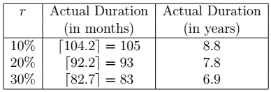
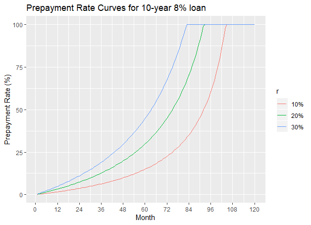
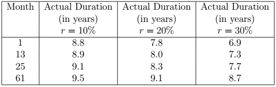
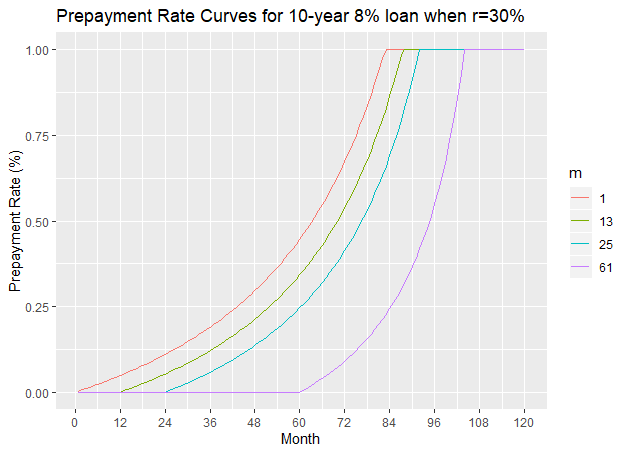
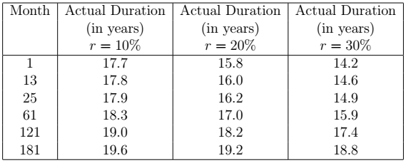
Let us consider some examples of loans and different scenarios of . We calculate the actual duration of the loan and plot prepayment rate curves which display the prepayment rates at different time points. Consider a loan with an interest rate of  and an initial duration of 10 years (). We consider three values of : 10%, 20% and 30%. The next table gives the actual duration (using Result 2) of the loan given a particular value of .
 values
The next figure shows the prepayment curves for the 10-year 8% loan when takes on values 10%, 20% and 30%.
Prepayment curve of a 10-year 8% loan
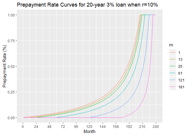
Consider a loan with an interest rate of 3% and an initial duration of 20 years (). We consider three values of : 10%, 20% and 30%. The next table gives the actual duration of this loan for the different values of and the next figure shows the prepayment curves.
 values
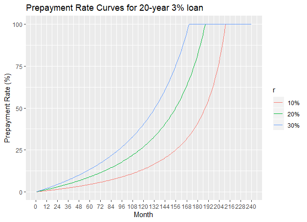
The increase in the repayment results in a faster rate of decrease in the outstanding principal. Hence the lender will actually receive less interest than initially expected. We can compare the Interest Component when prepayment is and is not present in order to calculate the reduction (loss) of interest income at each month for . We shall call the reducing in the interest at month : Interest Loss and given by formula:

where  is the expected interest income at month according to the repayment schedule, and
  is the actual interest income receive at month when prepayment is present.
Result 3: Consider a loan with associated principal , yearly interest rate compounded monthly and initial duration months. Let be the actual repayment amount where the value as calculated in equation (1). The loss of interest in the month is given by:
![\begin{equation*}\textup{Interest Loss}(k)=\begin{cases}rR[(1+\frac{i}{12})^{k-1}-1], & \textup{for }1\leq k \leq z\\R[1-(1+\frac{i}{12})^{k-n-1}], & \textup{for }z< k \leq n.\end{cases}\end{equation*}](https://datasciencegenie.com/wp-content/ql-cache/quicklatex.com-4413ca1aa7f9b780c7eeed9f552f7fd9_l3.png "Rendered by QuickLaTeX.com")
Proof: Let  .
.
![\begin{equation*}\begin{split}\textup{Interest Loss}(k)&=\textup{Interest Component}_{RS}(k)-\textup{Interest Component}_{Prep.}(k)\\&=[P(\frac{i}{12})(1+\frac{i}{12})^{k-1}-R(1+\frac{i}{12})^{k-1}+R]\\&\ \ \ -[P(\frac{i}{12})(1+\frac{i}{12})^{k-1}-(1+r)R(1+\frac{i}{12})^{k-1}+(1+r)R]\textup{ (by Lemmas 1(a) and 3a))}\\&=rR[(1+\frac{i}{12})^{k-1}-1].\end{split}\end{equation*}](https://datasciencegenie.com/wp-content/ql-cache/quicklatex.com-5c47f79bd7c4a86b030084ac321654ef_l3.png "Rendered by QuickLaTeX.com")
Let  .
.
![\begin{equation*}\begin{split}\textup{Interest Loss}(k)&=\textup{Interest Component}_{RS}(k)-\textup{Interest Component}_{Prep.}(k)\\&=[ P(\frac{i}{12})(1+\frac{i}{12})^{k-1}-R(1+\frac{i}{12})^{k-1}+R]-0 \textup{ (by Lemma 1(a))}\\&=R[1-(1+\frac{i}{12})^{-n}](1+\frac{i}{12})^{k-1}-R(1+\frac{i}{12})^{k-1}+R \textup{ (by Equation 1)}\\&=R[1-(1+\frac{i}{12})^{k-n-1}].\ \ \ \square\end{split}\end{equation*}](https://datasciencegenie.com/wp-content/ql-cache/quicklatex.com-26c58e8f3f09499713ef9a0079a62db2_l3.png "Rendered by QuickLaTeX.com")
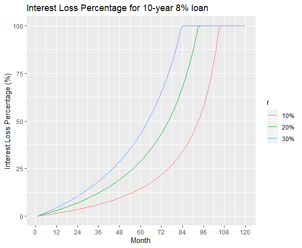
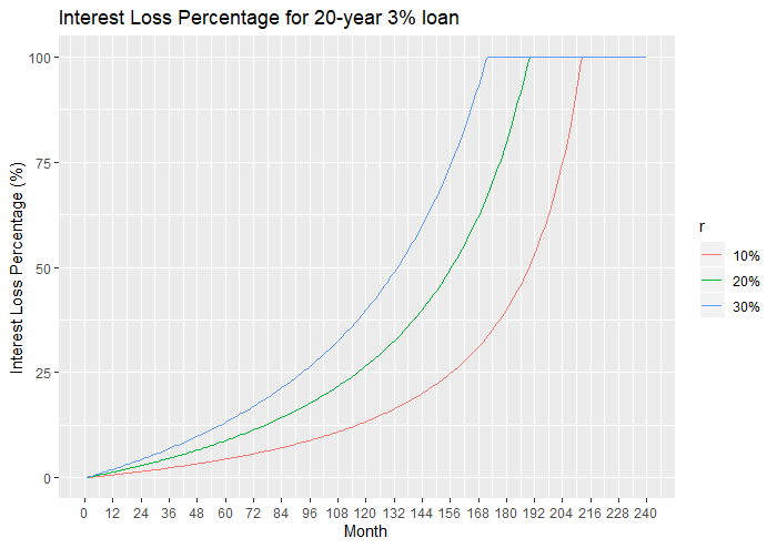
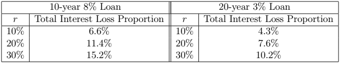
We can consider the fraction of the interest loss from the expected amount of interest receivable. We shall call this the Interest Loss Percentage, which is independent of the principal amount . The Interest Loss Percentage at the  month is given by formula:

The values  can be expressed as a function of the loan parameters as follows.
Result 4: Consider a loan with associated principal , yearly interest rate compounded monthly and initial duration months. Let be the actual repayment amount where the value as calculated in Equation (1). The percentage of loss of interest in the month is given by:
![\begin{equation*}\textup{Interest Loss Percentage}(k)=\begin{cases}\frac{r[(1+\frac{i}{12})^{k-1}-1]}{1-(1+\frac{i}{12})^{k-n-1}}\times 100\%, & \textup{for }1\leq k \leq z\\100\%, & \textup{for }z< k \leq n.\end{cases}\end{equation*}](https://datasciencegenie.com/wp-content/ql-cache/quicklatex.com-a60425e7c514034749ac6d9d433e9fa8_l3.png "Rendered by QuickLaTeX.com")
The next figures show the plots of Interest Loss Percentage for two loans: a 10-year 8% loan and a 20-year 3% loan. The curves all start at a value of 0% at month 1. Then they increase to 100% at time when the loan is repaid in full prematurely.
Let us consider the total interest paid on the loan in the case of having prepayments starting from the first month.
![\begin{equation*} \begin{split} \textup{Total Interest Paid}&=\sum_{k=1}^{z} \textup{Interest Component}(k)\\ &=\frac{P}{1-(1+\frac{i}{12})^{-n}}[(r+(1+\frac{i}{12})^{-n})(1-(1+\frac{i}{12})^z)+(1+r)(\frac{i}{12}) z]. \end{split} \end{equation*}](https://datasciencegenie.com/wp-content/ql-cache/quicklatex.com-dde806bc4697ccccba93583e35e9cea6_l3.png "Rendered by QuickLaTeX.com")
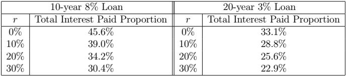
The fraction of the Total Interest Paid over the Principal amount is thus given by:

The next table gives the Total Interest Paid Proportion for the 10-year 8% loan and the 20-year 3% loan, for different values of . Note that =0% is the case when there is no prepayment present. The total interest paid proportion is inversely related to .
We can also calculate the Total Interest Loss which is the total interest which is lost on a loan due to prepayments. This can be calculated in two ways: either by summing all the values of  for or else by deducting the sum of the interest components when prepayment is present from the sum of interest components when prepayment is not present.

The Total Interest Loss on an loan whose prepayments start in the first month is given by:
![\begin{equation*} \textup{Total Interest Loss}=\frac{P}{1-(1+\frac{i}{12})^{-n}}[r(1+\frac{i}{12})^z+(1+\frac{i}{12})^{z-n}+\frac{i}{12}n-r-(1+r)(\frac{i}{12})z-1] \end{equation*}](https://datasciencegenie.com/wp-content/ql-cache/quicklatex.com-f03e53e964883676ab6559e40b0fb47f_l3.png "Rendered by QuickLaTeX.com")
The Total Interest Loss Proportion is thus given by:

The next Table gives the Total Interest Loss Proportion for the 10-year 8% loan and the 20-year 3% loan, for different values of .
Constant Prepayment from Month 
Suppose now that the prepayments start from month , that is, the monthly repayment is till month  and increases to from month onwards. The interest and capital components from the
  month repayment onwards change as follows.
Lemma 4: Consider a loan with associated principal , yearly interest rate compounded monthly and duration months. Let be the amount repaid monthly until month , as calculated in equation (1). Let be the monthly repayment amount from month onwards. Let be the actual duration of the loan, given that prepayment is present. The interest and capital component in the repayment and the outstanding principal at month , for  are given by:
![\begin{equation*}\begin{split}\textup{Interest Component}(k) &= P(\frac{i}{12})(1+\frac{i}{12})^{k-1}-R(1+\frac{i}{12})^{k-1}+R+rR[1-(1+\frac{i}{12})^{k-m}] \textup{ (a)}\\\textup{Capital Component}(k) &= R(1+\frac{i}{12})^{k-1}-P(\frac{i}{12})(1+\frac{i}{12})^{k-1}+rR(1+\frac{i}{12})^{k-m} \textup{ (b)}\\\textup{Principal}(k)&=P(1+\frac{i}{12})^k-\frac{R(1+\frac{i}{12})^k}{(\frac{i}{12})}+\frac{R}{(\frac{i}{12})}+\frac{rR[1-(1+\frac{i}{12})^{k-m+1}]}{(\frac{i}{12})} \textup{ (c)}\end{split}\end{equation*}](https://datasciencegenie.com/wp-content/ql-cache/quicklatex.com-1007aecf86d3a1f82733256e06856893_l3.png "Rendered by QuickLaTeX.com")
Proof: By induction on .
The next result gives the prepayment rate at each month.
Result 3: Consider a loan with associated principal , yearly interest rate compounded monthly and duration months. Let be the amount repaid monthly until month , as calculated in equation (1). Let be the monthly repayment amount from month onwards. Let be the actual duration of the loan, given that prepayment is present. The prepayment rate at month for  is 0, whilst the prepayment rate at month for is:
![\begin{equation*}\textup{Prepayment Rate}(k)=\frac{r[(1+\frac{i}{12})^{k-m+1}-1]}{1-(1+\frac{i}{12})^{k-n}}.\end{equation*}](https://datasciencegenie.com/wp-content/ql-cache/quicklatex.com-9e4ea314a0256e83d12de5dd221fab99_l3.png "Rendered by QuickLaTeX.com")
Proof: The proof is similar to that of Result 1.
Note that Result 1 can now be viewed as a corollary of Result 3 obtained by fixing to be 1. The next result gives a formula for the actual duration of a loan.
Result 4: Consider a loan with associated principal , yearly interest rate compounded monthly and duration months. When the actual monthly repayment is increased by a factor of from month onwards, the actual duration of the loan is:
![\begin{equation*}\lceil \frac{\ln{(1+r)}-\ln{[r(1+\frac{i}{12})^{1-m}+(1+\frac{i}{12})^{-n}]}}{\ln{(1+\frac{i}{12})}} \rceil\end{equation*}](https://datasciencegenie.com/wp-content/ql-cache/quicklatex.com-10126c62e96c32e62050b2ef45348bda_l3.png "Rendered by QuickLaTeX.com")
Proof: The proof is similar to that of Result 2.
At month , the loan is paid in full, and hence the prepayment rate at month is equal to 1. In fact, at month , we have:
![\begin{equation*} \begin{split} \textup{Interest Component}(z) &=P(\frac{i}{12})(1+\frac{i}{12})^{z-1}-R(1+\frac{i}{12})^{z-1}+R+rR[1-(1+\frac{i}{12})^{z-m}] \\ \textup{Capital Component}(z) &=\textup{Principal}(z-1)=P(1+\frac{i}{12})^{z-1}-\frac{R(1+\frac{i}{12})^{z-1}}{(\frac{i}{12})}+\frac{R}{(\frac{i}{12})}+\frac{rR[1-(1+\frac{i}{12})^{z-m}]}{(\frac{i}{12})}\\ \textup{Principal}(z)&=0. \end{split} \end{equation*}](https://datasciencegenie.com/wp-content/ql-cache/quicklatex.com-c7dfcd4a9292b2acc5f43cd3ffadc640_l3.png "Rendered by QuickLaTeX.com")
Adding the interest and capital component gives us the repayment amount:
![\begin{equation*} \frac{R}{\frac{i}{12}}[(1+r)(1+\frac{i}{12})-(1+\frac{i}{12})^{z-n}-r(1+\frac{i}{12})^{z-m+1}-(1+\frac{i}{12})^z] \end{equation*}](https://datasciencegenie.com/wp-content/ql-cache/quicklatex.com-ccdb7943f3c95bdb4c7fd5580d4837a0_l3.png "Rendered by QuickLaTeX.com")
This is the last repayment amount which is smaller or equal to that closes off the loan.
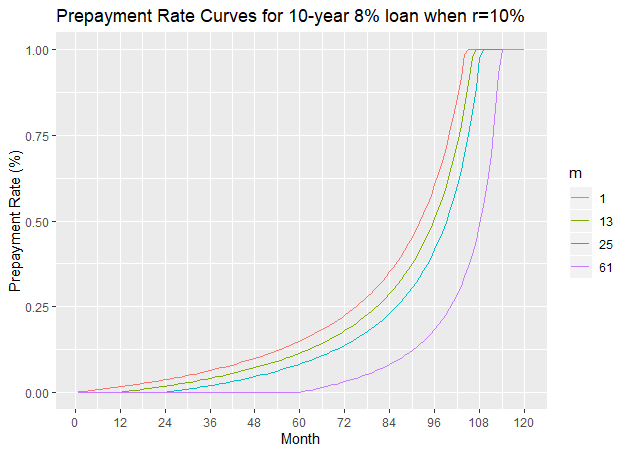
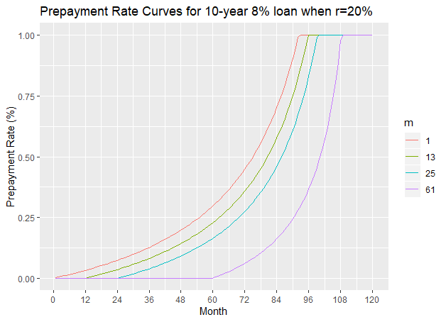
Consider a 10-year 8% loan. The next table gives the actual duration of the loan given an increase of in the repayments, starting from month . For simplicity,we consider only five case: the case when the increase in repayments starts from the first the repayment, after 1 year of repayments, after 2 years of repayments and after 5 years of repayments.
 and values
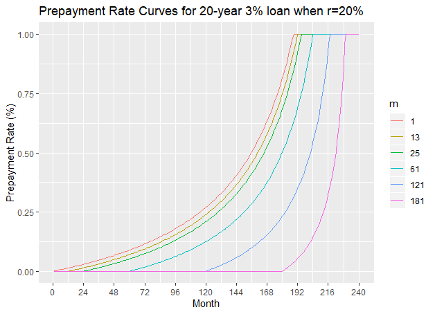
The next three figures show the prepayment curves for the 10-year 8% loan when =10%, 20% and 30% respectively, with various values of .
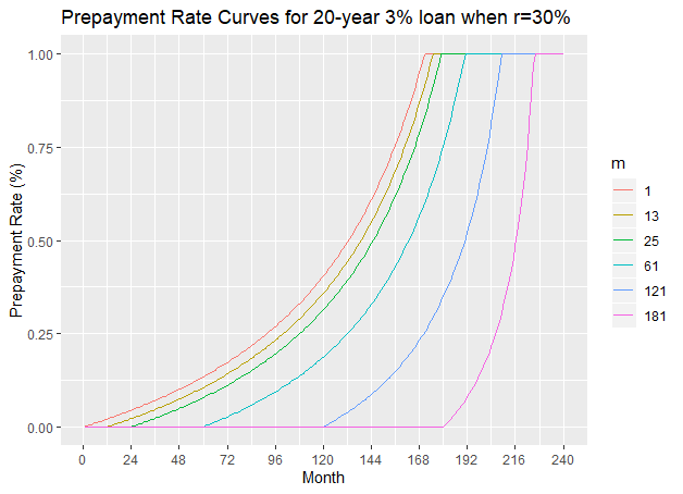
Consider a 20-year  loan. The next table gives the actual duration of the loan given an increase of in the repayments, starting from month . For simplicity, we consider only five case: the case when the increase in repayments starts from the first the repayment, after 1 year of repayments, after 2 years of repayments, after 5 years of repayments, after 10 years of repayments, and after 15 years of repayments.
 and values
The next three figures show the prepayment curves for the 20-year 3% loan when =10%, 20% and 30% respectively.
We can also calculate the loss of interest income, when the prepayment starts at month .
Result 7: Consider a loan with associated principal , yearly interest rate compounded monthly and initial duration months. Let be the amount repaid monthly till month and let be the actual repayment amount from month onwards, where the value as calculated in Equation (1). The loss of interest in the month is given by:
![\begin{equation*}\textup{Interest Loss}(k)=\begin{cases} 0, & \textup{for }k<m\\rR[(1+\frac{i}{12})^{k-m}-1], & \textup{for }m\leq k \leq z\\R[1-(1+\frac{i}{12})^{k-n-1}], & \textup{for }z< k \leq n.\end{cases}\end{equation*}](https://datasciencegenie.com/wp-content/ql-cache/quicklatex.com-13cc150a19b8943b651a5af2227bc06e_l3.png "Rendered by QuickLaTeX.com")
Proof: Similar to that of Result 3.
Alternatively, the Interest Loss at month could be represented by:
![\begin{equation*} \textup{Interest Loss}(k)=\max(0,\min(rR[(1+\frac{i}{12})^{k-m}-1],R[1-(1+\frac{i}{12})^{k-n-1}]))\mbox{ for }0\leq k \leq n. \end{equation*}](https://datasciencegenie.com/wp-content/ql-cache/quicklatex.com-407d4c71f075ef75f10401c71053fb36_l3.png "Rendered by QuickLaTeX.com")
The Interest Loss Percentage at the month is given by the following result.
Result 8: Consider a loan with associated principal , yearly interest rate compounded monthly and initial duration months. Let be the amount repaid monthly till month and let be the actual repayment amount from month onwards, where the value as calculated in Equation (1). The percentage of loss of interest in the month is given by:
![\begin{equation*}\textup{Interest Loss Percentage}(k)=\begin{cases} 0\%, & \textup{for }k<m\\\frac{r[(1+\frac{i}{12})^{k-m}-1]}{1-(1+\frac{i}{12})^{k-n-1}}\times 100\%, & \textup{for }m\leq k \leq z\\100\%, & \textup{for }z< k \leq n.\end{cases}\end{equation*}](https://datasciencegenie.com/wp-content/ql-cache/quicklatex.com-8b8e2d8d1e27ffb25a7934d5a8c3d851_l3.png "Rendered by QuickLaTeX.com")
Hence Results 3 and 4 can be viewed as special cases of Results 7 and 8 when  .
.
Let us consider the total interest paid on the loan in the case of having prepayments starting from the month.
![\begin{equation*} \begin{split} \textup{Total Interest Paid}&=\sum_{k=1}^{z} \textup{Interest Component}(k)\\ &=\frac{P}{1-(1+\frac{i}{12})^{-n}}[(1+\frac{i}{12})^{-n}-(1+\frac{i}{12})^{z-n}+(1+r)z(\frac{i}{12})-rm(\frac{i}{12})+r(1+\frac{i}{12})-r(1+\frac{i}{12})^{z-m+1}]. \end{split} \end{equation*}](https://datasciencegenie.com/wp-content/ql-cache/quicklatex.com-99c7900c3cd7a9b5db924be3f18550fc_l3.png "Rendered by QuickLaTeX.com")
The fraction of the Total Interest Paid over the Principal amount is thus given by:

The next two tables gives the Total Interest Paid Proportion for the 10-year 8% loan and the 20-year 3% loan, for different values of and . Note that =0% is the case when there is no prepayment present. Note that the higher the value and the earlier the repayments starts, the lower the Total Interest Rate Proportion.
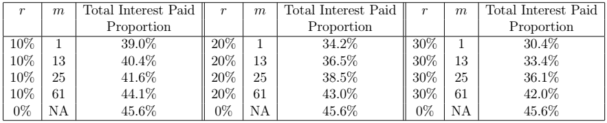 and
and 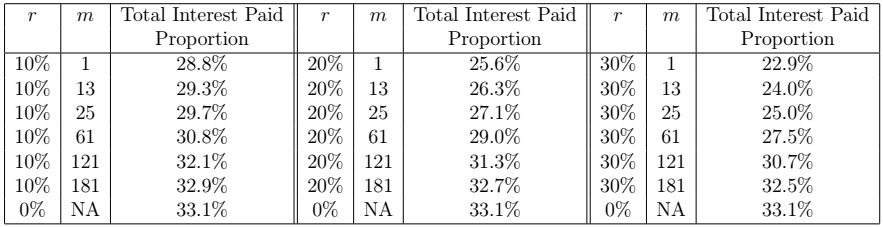 and
and Now we calculate the Total Interest Loss which is given by the following equation.
![\begin{equation*} \begin{split} \textup{Total Interest Loss}&=\sum_{k=1}^{n}\textup{Interest Loss}(k)=\textup{Total Interest Paid}_{RS}-\textup{Total Interest Paid}_{Prep.}\\ &=\frac{P}{1-(1+\frac{i}{12})^{-n}}[\frac{i}{12}n-1+(1+\frac{i}{12})^{z-n}-(1+r)z(\frac{i}{12})+rm(\frac{i}{12})-r(1+\frac{i}{12})+r(1+\frac{i}{12})^{z-m+1}]. \end{split} \end{equation*}](https://datasciencegenie.com/wp-content/ql-cache/quicklatex.com-b55c90996b5673912dd2cccdcbd12af7_l3.png "Rendered by QuickLaTeX.com")
The Total Interest Loss Proportion is thus given by:

The next tables give the Total Interest Loss Proportion for the 10-year 8% loan and the 20-year 3% loan, for different values of and .
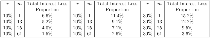 and
and 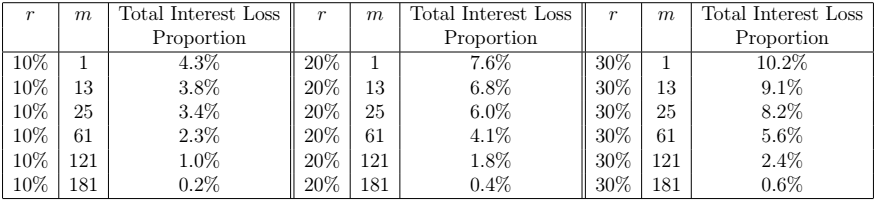 and
and Prepayment on a Portfolio of Loans
Suppose that we have a portfolio of  loans. A loan is initiated at time
  (that is the drawdown is at and the first repayment starts at
  ), has principal
  , yearly interest rate
  , and duration
  , for
, for  . Suppose that the time is a non-negative integer, set
  and let the time now be
  . Suppose that each repayment of each loan from time
  onwards is increased by a factor of . We would like to know the outstanding principal of the whole portfolio at each time from onwards, given that prepayment is present and compare it to that when prepayment is not present.
The outstanding principal of the whole portfolio  at time for
  , in the case where prepayment is not present is given by:
(3) 
where  is the outstanding principal of the
  loan at time .
Similarly, the outstanding principal of the whole portfolio  for
for  in the case when the prepayments start at is given by:
(4) ![\begin{equation*}\begin{split}\textup{Principal}_{\textup{Portfolio}}^{\textup{Prep.}}(k)=&\sum_{l=1}^{L} \textup{Principal}_l^{\textup{Prep.}}(k-k_l)\\=&\sum_{l=1}^{L} \max(0,P_l(1+\frac{i_l}{12})^{k-k_l}-\frac{R_l(1+\frac{i_l}{12})^{k-k_l}}{(\frac{i_l}{12})}+\frac{R_l}{(\frac{i_l}{12})})+\frac{rR_l[1-(1+\frac{i_l}{12})^{k-\kappa}]}{(\frac{i_l}{12})}) \textup{ using Lemma 4(c)}\end{split}\end{equation*}](https://datasciencegenie.com/wp-content/ql-cache/quicklatex.com-d9e5e859a7e20b9173dcc0862689d12f_l3.png "Rendered by QuickLaTeX.com")
where  is the outstanding principal of the loan at time .
We define the prepayment of the portfolio  at time as the sum of the extra capital repaid of each loan, at time . Thus for we have the equation:
(5) 
We define the prepayment rate of the portfolio of loans  at time as the sum of extra capital repaid of each loan divided by the total outstanding principal of the loans given that prepayment is not present:
(6) 
The expected inflow of interest income at month is sum of the interest components at month of all the loans of the portfolio, given that prepayment is not present. This is given by the equation:

The actual inflow of interest income at month is sum of the interest components at month of all the loans of the portfolio, given that prepayment is present. This is given by the equation:

for  , where
  is the interest component in the
  month of loan
  , given that prepayment starts from month
  .
.
The Interest Loss on the whole portfolio at time , for is given by:
![\begin{equation*} \begin{split} \textup{Interest Loss}_\textup{Portfolio}(k)&=\sum_{l=1}^{L} \textup{Interest Loss}_l(k-k_l)\times\chi_{\lbrace k -k_l\leq n_l\rbrace}\\ &=\sum_{l=1}^{L} \max(0,\min(rR_l[(1+\frac{i_l}{12})^{k-\kappa-1}-1],R_l[1-(1+\frac{i_l}{12})^{k-k_l-n_l-1}]))\times\chi_{\lbrace k -k_l\leq n_l\rbrace} \end{split} \end{equation*}](https://datasciencegenie.com/wp-content/ql-cache/quicklatex.com-f6b608944016d0ef9ded35de9a6088cb_l3.png "Rendered by QuickLaTeX.com")
where  is the interest loss on loan at month and
  if
if  or 0 otherwise.
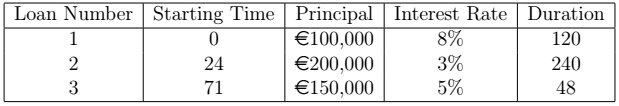
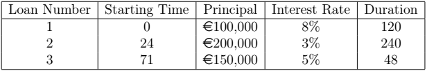
Consider the following example. Suppose we have a portfolio made up of three loans as characterised in the next table.
Let the time now be  and suppose that each repayment from time
  onwards increases by a factor of and we take to be equal to
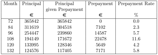
  as an example. The next table gives some results derived from Equations (3), (4), (5) and (6) respectively. Note that the month numbers are chosen at an interval of 12. So the row corresponding to 84 shows the state of the portfolio after a year of prepayments, the row corresponding to 96 shows the state of the portfolio after two years of prepayments and so on.
 =10%
=10%The next figure shows the portfolio prepayment rate curves for r=10%, 20% and 30%.
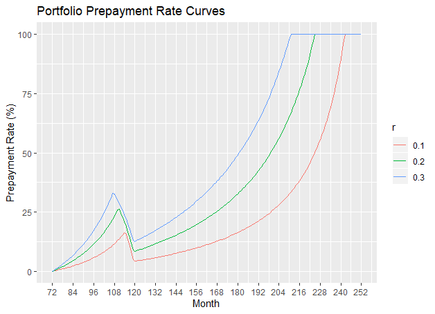 =10%, 20% and 30%
Consider the prepayment rate curve for =10%. This reaches a local maximum of 16.3% at month 114, which is the month before both Loan 1 and Loan 3 are repaid in full. It reaches a local minimum at month 120, by which time the outstanding principal of both Loan 1 and Loan 3 have reached an outstanding principal of 0 according to their respective repayment schedules (excluding prepayment). From that month onwards, the prepayment rate curve keeps on increasing to reach 100% at which time Loan 3 is repaid in full. Note that since the repayment schedule (excluding prepayment) is independent of , all the three prepayment rate curves reach a local minimum at month 120.
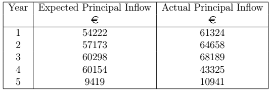
One could then derive the next table which shows the inflow of portfolio principal during the next five years. The expected principal inflow is the sum of the capital portion of each repayment during a particular year, while the actual principal inflow is the sum of the capital portion of each repayment during a particular year given that prepayment is present.
 =10%
=10%The next figure offers a visualisation of an extension of the data given in the previous table. It shows a plot of the expected and actual inflow of principal (for =10%) over the next 20 years.
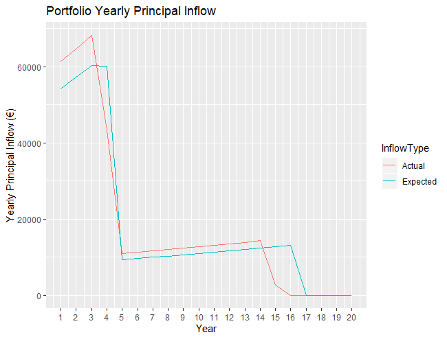 =10%
=10%Next we consider the expected and actual inflow of interest income. The next graph shows the monthly inflow of expected interest income and the actual interest income given the increase in the repayments of r=10%, 20% and 30%.
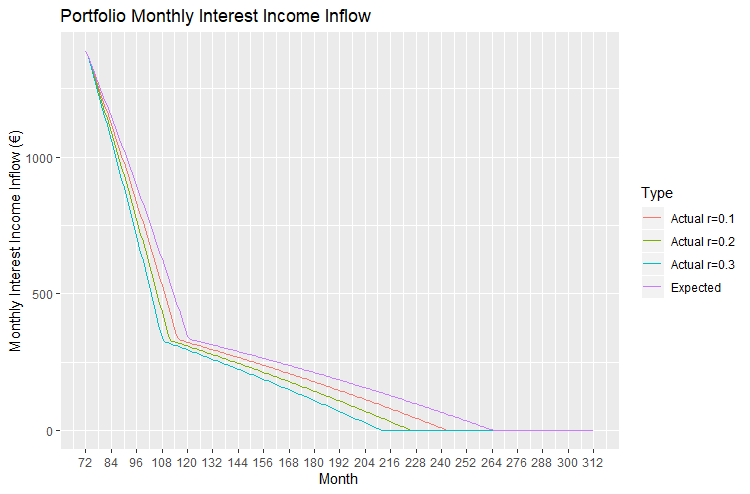
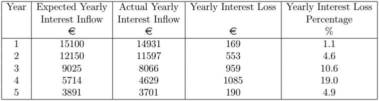
These monthly figures can be group in order to obtain the yearly expected and actual inflow of interest income. The next table gives the annual inflow of interest income, both expected and actual, during the next five years for =10%. Their difference results in the loss of interest income over a yearly basis. The loss can be expressed a percentage by computing the fraction of yearly interest loss over the expected yearly inflow of interest income.
 =10%
=10%Prepayment from a decrease in the interest rate
In what follows, we consider the prepayment in the loan resulting from a decrease in the interest rate whilst the monthly repayment is kept constant, and not revised according the new interest rate. We consider a loan with principal , interest rate and term months. Each monthly repayment will always be equal to as given by Equation (1) (even when prepayment is present). The interest rate will decrease to a lower new interest rate  . In the next section, we will consider the case when the change in interest rate happens exactly at the time of draw-down (at month 0). This will be generalised to the case when the change in the interest rate happens at any month .
Constant Prepayment from Month 1 resulting from a decrease in the interest rate
Let us assume that the interest rate changes from to exactly at the time of draw-down. Hence the borrower starts making prepayments from the first repayment (at month 1). We are after: (1) the prepayment rate at each month (2) the actual duration of the loan. First, from Lemma 5 we can deduce the capital component, the interest component and outstanding principal in this case.
Lemma 5: Consider a loan with associated principal , yearly interest rate compounded monthly and duration months. Let the interest rate be decreased to a new yearly interest rate . Let be the monthly repayment as calculated in Equation (1) and let be the actual duration of the loan, given that prepayment is present. The interest and capital component in the repayment and the outstanding principal at month , for are given by:

Proof: By induction on .
Result 9: Consider a loan with associated principal , yearly interest rate compounded monthly and duration months. Let the interest rate be decreased to at month 0. Then the prepayment rate at month , for is:
![\begin{equation*}\textup{Prepayment Rate}(k)=\frac{1-\frac{i}{i'}-(1+\frac{i}{12})^{k-n}+(1+\frac{i'}{12})^k[(1+\frac{i}{12})^{-n}+\frac{i}{i'}-1]}{1-(1+\frac{i}{12})^{k-n}}.\end{equation*}](https://datasciencegenie.com/wp-content/ql-cache/quicklatex.com-80f0e5a6d28356bbb9bd78e195361325_l3.png "Rendered by QuickLaTeX.com")
Proof:
![\begin{equation*}\begin{split}\text{Prepayment Rate}(k)&= \frac{\text{Principal}_{\text{RS}}(k)-\text{Principal}_{\text{Actual}}(k)}{\text{Principal}_{\text{RS}}(k)} \text{ (by Equation (2)})\\&=\frac{P(1+\frac{i}{12})^k-\frac{R(1+\frac{i}{12})^k}{(\frac{i}{12})}+\frac{R}{(\frac{i}{12})}-P(1+\frac{i'}{12})^k+\frac{R(1+\frac{i'}{12})^k}{(\frac{i'}{12})}-\frac{R}{(\frac{i'}{12})}}{P(1+\frac{i}{12})^k-\frac{R(1+\frac{i}{12})^k}{(\frac{i}{12})}+\frac{R}{(\frac{i}{12})}}\text{ (by Lemma 1(c) and Lemma 5(c))}\\&=\frac{1-\frac{i}{i'}-(1+\frac{i}{12})^{k-n}+(1+\frac{i'}{12})^k[(1+\frac{i}{12})^{-n}+\frac{i}{i'}-1]}{1-(1+\frac{i}{12})^{k-n}}. $\square$\end{split}\end{equation*}](https://datasciencegenie.com/wp-content/ql-cache/quicklatex.com-6ae3f775795a0be896143f471445cb11_l3.png "Rendered by QuickLaTeX.com")
Result 10: Consider a loan with associated principal , yearly interest rate compounded monthly and duration months. When the interest rate is decreased to at month 0, the actual duration of the loan is:
![\begin{equation*}z=\lceil \frac{\ln{\frac{i}{i'}}-\ln{[\frac{i}{i'}-1+(1+\frac{i}{12})^{-n}]}}{\ln{(1+\frac{i'}{12})}} \rceil\end{equation*}](https://datasciencegenie.com/wp-content/ql-cache/quicklatex.com-e0a7b3c308d6367b7af9951dc94a0b52_l3.png "Rendered by QuickLaTeX.com")
Proof: Let be the least integer such that the prepayment rate is greater or equal to 1. Then is the actual duration of the loan. Note that we assume that and hence .
![\begin{equation*}\begin{split}\text{Prepayment Rate}(k)&\geq 1\\\frac{1-\frac{i}{i'}-(1+\frac{i}{12})^{k-n}+(1+\frac{i'}{12})^k[(1+\frac{i}{12})^{-n}+\frac{i}{i'}-1]}{1-(1+\frac{i}{12})^{k-n}}&\geq 1\text{ (by Result 9)}\\(1+\frac{i'}{12})^k[(1+\frac{i}{12})^{-n}+\frac{i}{i'}-1]-\frac{i}{i'} & \geq 0\\(1+\frac{i'}{12})^k &\geq \frac{\frac{i}{i'}}{\frac{i}{i'}-1+(1+\frac{i}{12})^{-n}}\\k&\geq \frac{\ln{\frac{i}{i'}}-\ln{[\frac{i}{i'}-1+(1+\frac{i}{12})^{-n}]}}{\ln{(1+\frac{i'}{12})}}.\end{split}\end{equation*}](https://datasciencegenie.com/wp-content/ql-cache/quicklatex.com-37f25e5b159e7b79bfe2561b2f3ebd81_l3.png "Rendered by QuickLaTeX.com")
Hence result follows.
Note that Results 9 and 10 are independent of the principal . Note also that in the trivial case when  , the actual duration is equal to the initial duration . At month , the loan is paid in full, and hence the prepayment rate at month is equal to 1. In fact, at month , we have:

Adding the interest and capital component gives us the repayment amount:

This is the last repayment amount which is smaller or equal to that closes off the loan.
Let us consider some examples of loans and different scenarios of , for which we calculate the actual duration of the loan and plot prepayment rate curves.
Consider a loan with an initial interest rate  and an initial duration of 10 years (). Let the interest rate be changed to where
  ,
,  and
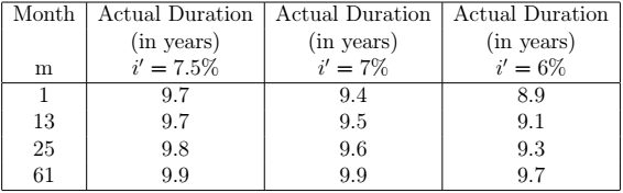
and  . The next table gives the actual duration (using Result 10) of the loan given these particular values of .
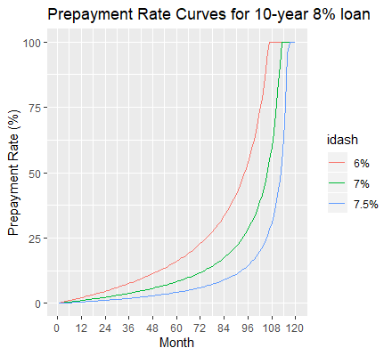
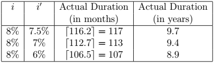 interest rate for various values
The next figure shows the prepayment curves for the 10-year 8% loan when takes on values 7.5%, 7% and 6%.
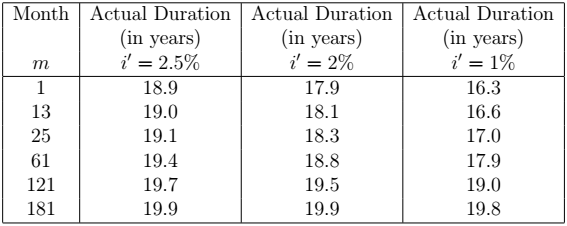
Consider a loan with an interest rate of and an initial duration of 20 years (). We consider three values of :  ,
,  and
and  . The next table gives the actual duration of this loan for the different values of and the next figure shows the corresponding prepayment curves.
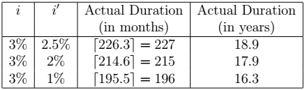 interest rate for various values
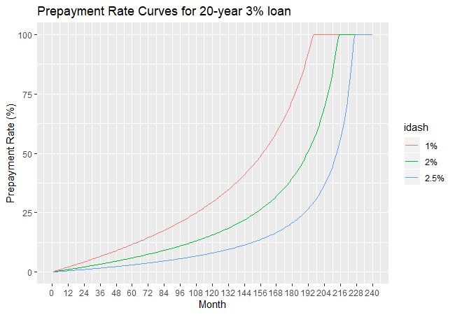 loan for various values of
 We calculate the interest income lost at each month resulting from the prepayments induced by the decrease in interest rate.
Result 11: Consider a loan with associated principal , yearly interest rate compounded monthly and initial duration months. Let be the repayment amount as calculated in Equation (1) and let the interest rate be decreased to at month 0. The loss of interest in the month is given by:
![\begin{equation*}\textup{Interest Loss}(k)=\begin{cases}R[(1+\frac{i'}{12})^{k-1}(1+\frac{i'}{i}(1+i/12)^{-n}-\frac{i'}{i})-(1+\frac{i}{12})^{k-n-1}], & \textup{for }1\leq k \leq z\\R[1-(1+\frac{i}{12})^{k-n-1}], & \textup{for }z< k \leq n.\end{cases}\end{equation*}](https://datasciencegenie.com/wp-content/ql-cache/quicklatex.com-7b5bfd510dd1d838e78fcc787df6645d_l3.png "Rendered by QuickLaTeX.com")
Proof: Similar to that of Result 3.
We can consider the fraction of the interest loss from the expected amount of interest receivable. We calculate Interest Loss Percentage, which is the fraction of the interest loss from the expected amount of interest receivable.
Result 12: Consider a loan with associated principal , yearly interest rate compounded monthly and initial duration months. Let be the repayment amount as calculated in Equation (1) and let the interest rate be decreased to at month 0. The percentage of loss of interest in the month is given by:

The next two figures show the plot of Interest Loss Percentage for two loans: a 10-year loan and a 20-year loan. The curves all start at a value of  at month 1. Then they increase to 100
 at time when the loan is repaid in full prematurely.
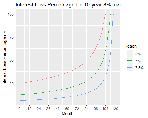
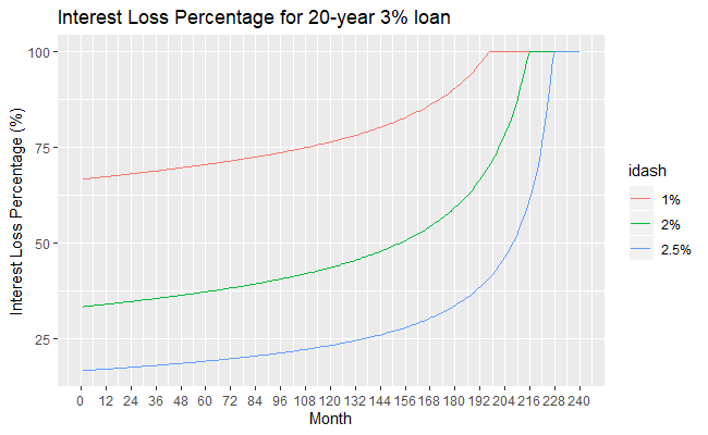
Interest Loss Percentage in the repayments of a 10-year loan and a 20-year loan respectively
Let us consider the total interest paid on the loan in the case of having prepayments starting from the first month.
![\begin{equation*}\begin{split}\textup{Total Interest Paid}&=\sum_{k=1}^{z} \textup{Interest Component}(k)\\&=\frac{P[((1+\frac{i'}{12})^z-1)(1-(1+\frac{i}{12})^{-n})+\frac{i}{i'}(1-(1+\frac{i'}{12})^z)+\frac{i}{12}z]}{1-(1+\frac{i}{12})^{-n}}.\end{split}\end{equation*}](https://datasciencegenie.com/wp-content/ql-cache/quicklatex.com-58be5f4ba002f1000d71dfdde08017f4_l3.png "Rendered by QuickLaTeX.com")
The fraction of the Total Interest Paid over the Principal amount is thus given by:

The next table gives the Total Interest Paid Proportion for the 10-year loan and the 20-year loan, for different values of . For comparison we show the total interest paid proportion for the case when  , that is, when no prepayment present.
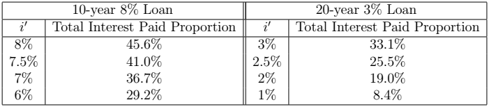 Loan and 20-year Loan
The Total Interest Loss which is the total interest which is lost on a loan due to prepayments is given by the following formula.
![\begin{equation*}\begin{split}\textup{Total Interest Loss}&=\sum_{k=1}^{n}\textup{Interest Loss}(k)=\textup{Total Interest Paid}_{RS}-\textup{Total Interest Paid}_{Prep.}\\&=\frac{P[\frac{i}{12}(n-z)+(1+\frac{i'}{12})^{z}((1+\frac{i}{12})^{-n}+\frac{i'}{i}-1)-\frac{i}{i'}]}{1-(1+\frac{i}{12})^{-n}}.\end{split}\end{equation*}](https://datasciencegenie.com/wp-content/ql-cache/quicklatex.com-02fe17059310ee7fd6138f2f6268d5ac_l3.png "Rendered by QuickLaTeX.com")
The Total Interest Loss Proportion is thus given by:

The next table gives the Total Interest Loss Proportion for the 10-year loan and the 20-year loan, for different values of .
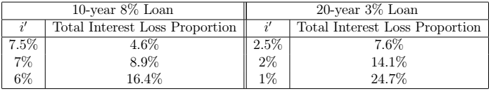 Loan and 20-year Loan
Constant Prepayment from Month resulting from a decrease in the interest rate
Suppose now that the decrease in the interest rate happens exactly at the time of the  repayment, that is, at month . Hence the prepayments start from month . The interest and capital components from the month repayment onwards change as follows.
Lemma 6: Consider a loan with associated principal , yearly interest rate compounded monthly and duration months. Let be the amount repaid monthly as calculated in Equation (1) and let the interest rate be decreased to at month . Let be the actual duration of the loan, given that prepayment is present. The interest and capital component in the repayment and the outstanding principal at month , for are given by:

where
 is the outstanding principal at month given by
  .
.
Proof: By induction on .
Result 13 gives the prepayment rate at each month.
Result 13: Consider a loan with associated principal , yearly interest rate compounded monthly and duration months. Let be the amount repaid monthly as calculated in Equation (1) and let the interest rate be decreased to at month . Let be the actual duration of the loan, given that prepayment is present. The prepayment rate at month for is 0, whilst the prepayment rate at month for is:

Proof: The proof is similar to that of Result 1.
Note that Result 9 can now be viewed as a corollary of Result 13 obtained by fixing to be 1. Result 14 gives a formula for the actual duration .
Result 14: Consider a loan with associated principal , yearly interest rate compounded monthly and duration months. When the interest rate is decreased to at month , the actual duration of the loan is:

\end{result}
Proof: The proof is similar to that of Result 2.
Result 10 can now be seen as a corollary of Result 14 for the case when .
At month , the loan is paid in full, and hence the prepayment rate at month is equal to 1. In fact, at month , we have:

Adding the interest and capital component gives us the repayment amount:
![\begin{equation*}R[(\frac{1}{(\frac{i}{12})}-\frac{1}{(\frac{i'}{12})}-\frac{(1+\frac{i}{12})^{m-n-1}}{(\frac{i}{12})})(1+\frac{i'}{12})^{z-m+1}+1+\frac{1}{(\frac{i'}{12})}]\end{equation*}](https://datasciencegenie.com/wp-content/ql-cache/quicklatex.com-91958026868a322286072b8a03cc9a5a_l3.png "Rendered by QuickLaTeX.com")
This is the last repayment amount which is smaller or equal to that closes off the loan.
Consider a 10-year loan. The next table gives the actual duration of the loan given a change of interest rate to at month . For simplicity, we consider only five case: the case when the prepayments start from the first the repayment, after 1 year of repayments, after 2 years of repayments and after 5 years of repayments.
 interest rate for various and values
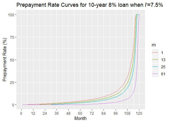
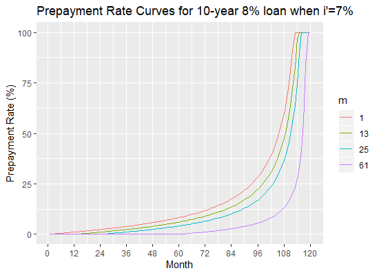
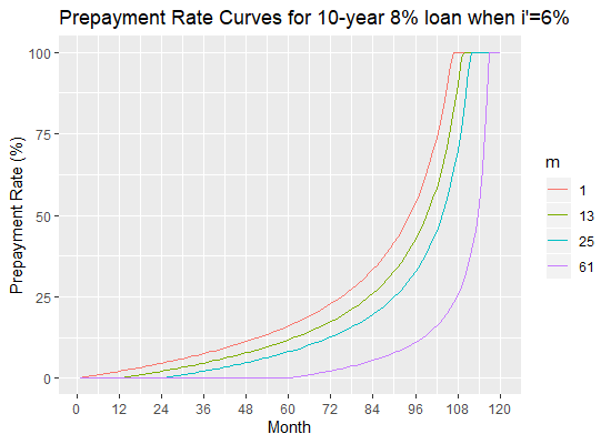
The next three figures show the prepayment curves for the 10-year 8\% loan when i’=7.5\%, 7\% and 6\% respectively, with various values of .
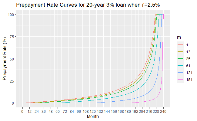
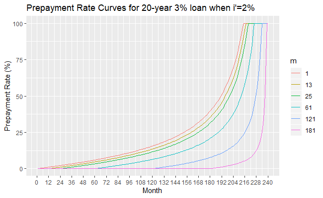
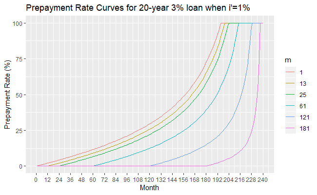
Consider a 20-year loan. The next table gives the actual duration of the loan given a decrease in the interest rate decrease to in month . For simplicity, we consider only five case: the case when the prepayment starts from the first the repayment, after 1 year of repayments, after 2 years of repayments, after 5 years of repayments, after 10 years of repayments, and after 15 years of repayments.
 interest rate for various and values
The next three figures show the prepayment curves for the 20-year 3\% loan when  and respectively.
We can also calculate the loss of interest income, when the prepayment starts at month .
Result 15: Consider a loan with associated principal , yearly interest rate compounded monthly and initial duration months. Let be the amount repaid monthly as calculated in Equation (1) and let the interest rate be decreased to at month . The loss of interest in the month is given by:
![\begin{equation*}\textup{Interest Loss}(k)=\begin{cases} 0, & \textup{for }k<m\\R[(1+\frac{i'}{12})^{k-m}(1-\frac{i'}{i}+(\frac{i'}{i})(1+\frac{i}{12})^{m-n-1})-(1+\frac{i}{12})^{k-n-1}], & \textup{for }m\leq k \leq z\\R[1-(1+\frac{i}{12})^{k-n-1}], & \textup{for }z< k \leq n.\end{cases}\end{equation*}](https://datasciencegenie.com/wp-content/ql-cache/quicklatex.com-e7daeef55881ad54505b72a815d0607c_l3.png "Rendered by QuickLaTeX.com")
Proof: Similar to that of Result 3.
The Interest Loss Percentage at the month is given by the following result.
Result 16: Consider a loan with associated principal , yearly interest rate compounded monthly and initial duration months. Let be the amount repaid monthly as calculated in Equation (1) and let the interest rate be decreased to at month . The percentage of loss of interest in the month is given by:

\end{result}
Hence Results 11 and 12 can be viewed as special cases of Results 15 and 16 when .
Let us consider the total interest paid on the loan in the case of having prepayments starting from the month.
![\begin{equation*}\begin{split}\textup{Total Interest Paid}&=\sum_{k=1}^{z} \textup{Interest Component}(k)\\&=\frac{P}{1-(1+\frac{i}{12})^{-n}}[z(\frac{i}{12})+(1+\frac{i}{12})^{-n}-1+\frac{i}{i'}+(1-(1+\frac{i}{12})^{m-n-1}-\frac{i}{i'})(1+\frac{i'}{12})^{z-m+1}].\end{split}\end{equation*}](https://datasciencegenie.com/wp-content/ql-cache/quicklatex.com-2bf4c44c568db216be54b8814b7f2136_l3.png "Rendered by QuickLaTeX.com")
The fraction of the Total Interest Paid over the Principal amount is thus given by:

The next two tables give the Total Interest Paid Proportion for the 10-year 8\% loan and the 20-year 3\% loan respectively, for different values of and . Note that  is the case when there is no prepayment present. Note that the lower the value and the earlier the repayments starts, the lower the Total Interest Rate Proportion.
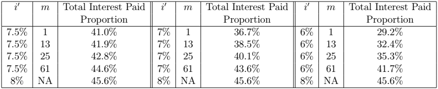 Loan for various and values
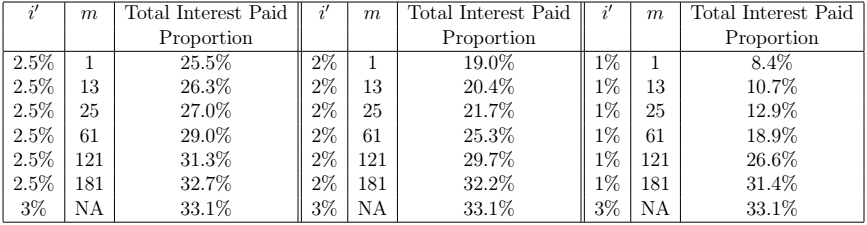 Loan for various and values
Now we calculate the Total Interest Loss which is given by the following equation.
![\begin{equation*}\begin{split}\textup{Total Interest Loss}&=\sum_{k=1}^{n}\textup{Interest Loss}(k)=\textup{Total Interest Paid}_{RS}-\textup{Total Interest Paid}_{Prep.}\\&=\frac{P}{1-(1+\frac{i}{12})^{-n}}[(n-z)(\frac{i}{12})-\frac{i}{i'}-(1-(1+\frac{i}{12})^{m-n-1}-\frac{i}{i'})(1+\frac{i'}{12})^{z-m+1}].\end{split}\end{equation*}](https://datasciencegenie.com/wp-content/ql-cache/quicklatex.com-b6dbaa947a96b0d45784a96a89ea958e_l3.png "Rendered by QuickLaTeX.com")
The Total Interest Loss Proportion is thus given by:

The next two tables give the Total Interest Loss Proportion for the 10-year loan and the 20-year loan respectively, for different values of and .
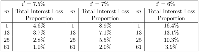 Loan for various and values
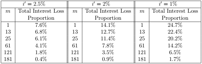 Loan for various and values
Prepayment on a Portfolio of Loans resulting from a decrease in the interest rates
Suppose that we have a portfolio of loans. A loan is initiated at time (that is the drawdown is at and the first repayment starts at ), has principal , yearly interest rate , and duration , for . Suppose that the time is a non-negative integer, set and let the time now be . Suppose that at the time now, , the interest rates change from to  , . Hence prepayments starts with the repayments at time . We would like to know the outstanding principal of the whole portfolio at each time from onwards, given that prepayment is present and compare it to that when prepayment is not present.
The outstanding principal of the whole portfolio at time for , in the case where prepayment is not present is given by Equation (3). On the other hand, the outstanding principal of the whole portfolio for in the case when the prepayments start at , due to a decrease in the interest rates at time , is given by:
(7) 
where is the outstanding principal of the loan at time given that the interest rate decreases to  at the
  repayment time, and
  .
.
The prepaid amount and the prepayment rate of the portfolio at time are obtained by substituting Equation (7) in Equations (5) and (6) respectively.
Recall that the expected inflow of interest income at month (that is the case in which prepayment is not present) is given by:

The actual inflow of interest income at month , given a decrease in the interest rates is given by the equation:

for  , where is the interest component in the month of loan , given that interest rate decreases to at month
  and .
and .
The Interest Loss on the whole portfolio at time , for is the difference between  and
and  .
.
Consider the following example. Suppose we have a portfolio made up of three loans as characterised in the next table.
Let the time now be and at the time now, the interest rates of all the loans in the portfolio and decreased by . Hence the interest rate of Loan 1 changes to ( ), the interest rate of Loan 2 changes to (
 ) and the interest rate of Loan 3 changes to
  (
( ). This will lead to prepayments from time onwards.
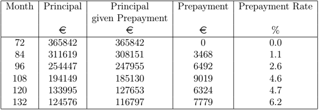
The next table gives some results derived from Equations (3), (7), (5) and (6). Note that the month numbers are chosen at an interval of 12. So the row corresponding to 84 shows the state of the portfolio after a year of prepayments, the row corresponding to 96 shows the state of the portfolio after two years of prepayments and so on.
The next figure shows the portfolio prepayment rate curves when the interest rates are decreased by  , and .
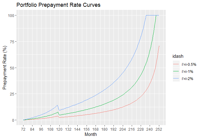 , , and
 Consider the prepayment rate curve resulting from a decrease of in the interest rates. This reaches a local maximum of 7.6\% at month 118, which is the month before both Loan 1 and Loan 3 are repaid in full. It reaches a local minimum at month 120, by which time the outstanding principal of both Loan 1 and Loan 3 have reached an outstanding principal of 0 according to their respective repayment schedules (excluding prepayment). From that month onwards, the prepayment rate curve keeps on increasing to reach 100\% at which time Loan 3 is repaid in full. Note that since the repayment schedule (excluding prepayment) is independent of  , all the three prepayment rate curves reach a local minimum at month 120.
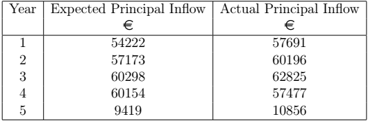
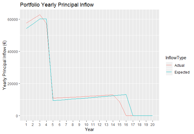
One could then derive the inflow of portfolio principal during the next five years, shown in the next table. The expected principal inflow is the sum of the capital portion of each repayment during a particular year, while the actual principal inflow is the sum of the capital portion of each repayment during a particular year given that prepayment is present.
The next figure displays the extension of the data presented in the above table to 20 years.
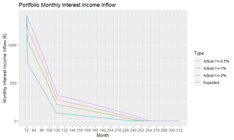
Next we consider the expected and actual inflow of interest income. The next figure shows the monthly inflow of expected interest income and the actual interest income given the increase a decrease in the interest rates by , and .
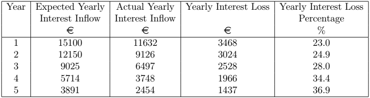
These monthly figures can be group in order to obtain the yearly expected and actual inflow of interest income. The next table gives the annual inflow of interest income, both expected and actual, during the next five years for the case when the interest rates are decreased by . Their difference results in the loss of interest income over a yearly basis. The loss can be expressed a percentage by computing the fraction of yearly interest loss over the expected yearly inflow of interest income.
Conclusion
We studied the effects of prepayments on a loan, resulting from two different scenarios. The first scenario is when the repayments are increased by some factor from one time point onwards. The second scenario is when the interest rate of the loan is decreased at some time point whilst the monthly repayment amount remains unchanged. Both instances result in prepayment on the loan due to premature repayment of the principal. For each scenario, we found closed formulae for the actual duration of the loan and the prepayment rate of the loan at each month. Moreover a formula is obtained to quantify the interest income lost due to the prepayment.
All of this was combined in order to study a portfolio of loans. We obtain the prepayment rate of the whole portfolio and constructed prepayment rate graphs. We computed the actual outstanding (combined portfolio) principal given the presence of prepayment and compared it to the expected outstanding principal. This is useful for the asset-liability management of the lending institution. The actual interest income inflow from the portfolio of loans is also calculated. This can also be used as a risk assessment measure of the future income of the lending institution.