Latin Hypercube Sampling vs. Monte Carlo Sampling

Introduction

Monte Carlo Sampling (MCS) and Latin Hypercube Sampling (LHS) are two methods of sampling from a given probability distribution. In MCS we obtain a sample in a purely random fashion whereas in LHS we obtain a pseudo-random sample, that is a sample that mimics a random structure. In order to give a rough idea, MC simulation can be compared to simple random sampling whereas Latin Hypercube Sampling can be compared to stratified sampling. Suppose we want to pick 20 people from a city which has 5 districts. In random sampling the 20 people are chosen randomly (without the use of any structured method) and in stratified sampling, 4 people are chosen randomly from each of the 5 districts.

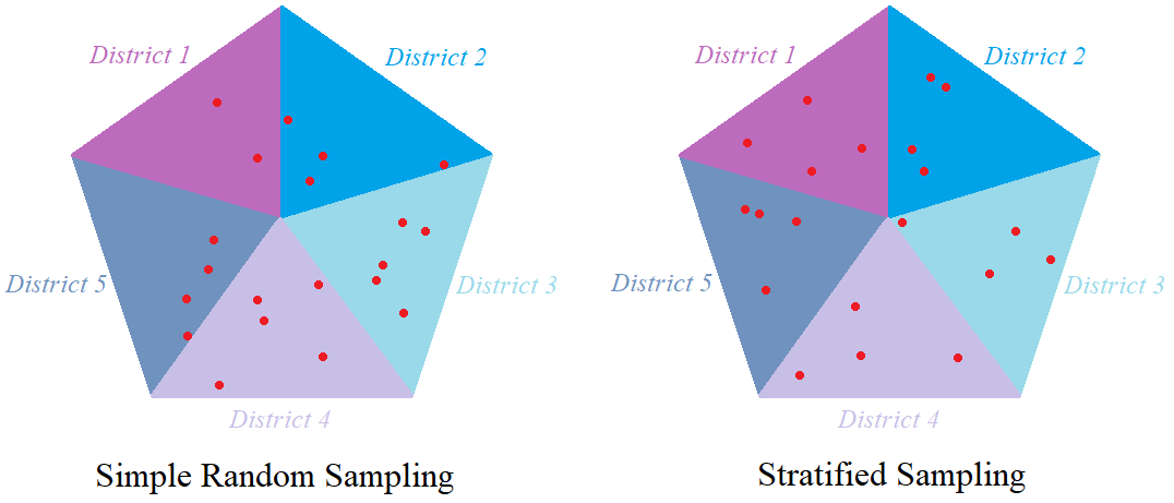
The advantage of stratified sampling over simple random sampling is that even though it is not purely random, it requires a smaller sample size to attain the same precision of the simple random sampling. We will see something similar when simulating using MCS and LHS. Both methods are explained and the R code for generating samples is provided for each method. The methods are compared with each other in terms of convergence. The two sampling methods are then extended to and demonstrated on bivariate cases, for which the rate of convergence is also analysed.

Monte Carlo Sampling

Suppose that we have a random variable $X$ with a probability density function $f(x)$ and cumulative distribution function $F(x)$ . We would like to generate a random sample of $n$ values from this distribution. Let us generate the first value. We generate a random number between 0 and 1 and call it $u$ (that is $u$ is uniformly-distributed on the interval [0,1]). The value $F^{-1}(u)$ where $F^{-1}$ is the inverse of the cumulative distribution function $F$ , is our first sample point, which we call $x$ . Note that by using mathematical theory, it can be shown that $x=F^{-1}(u)$ has its probability density function equal to $f(x)$ .

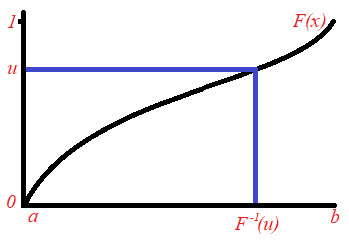
This process is repeated until we have gathered $n$ values for our sample. The idea of generating a uniformly-distributed random value and converting it using $F^{-1}$ in order to follow the desired distribution is called the Analytical Inversion Method. For more information, one can have a look here at the article that compares the Analytical Inversion Method to an alternative method known as the Accept-Reject Method.

Latin Hypercube Sampling

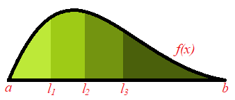
Consider a random variable $X$ with probability density function $f(x)$ and cumulative distribution function $F(x)$ . We would like to sample $n$ values from this distribution using LHS. The idea is to split the total area under the probability density function into $n$ portions that have equal area. Since the total area under the probability density function is 1, each portion would have an area of $\frac{1}{n}$ . We take a random value from each portion. This will give us a sample of $n$ values.

The next diagram displays this idea. It shows an example of a probability density function whose domain is $[a,b]$ and the area is split into 4 segments. In general this idea works even when the domain is unbounded (for example, in the case of the normal distribution where the values $X$ can take could be anything from $-\infty$ to $\infty$ ). Moreover the number of segment, that is, the sample size, could be any positive integer. In this particular case, we would obtain one number from each interval: $[a,l_1), [l_1,l_2), [l_2,l_3)$ and $[l_3,b]$ .

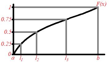
This is carried out by using the Analytical Inversion Method. In general, the interval $[0,1]$ is split into $n$ equal segments $[0,\frac{1}{n}), [\frac{1}{n},\frac{2}{n}),\cdots,[\frac{n-1}{n},1]$ . We generate a uniformly-distributed random variable from each of these $n$ intervals and obtain $u_1,u_2,\cdots,u_n$ . Then our resultant sample becomes $x_1,x_2,\cdots,x_n$ where $x_1=F^{-1}(u_1), x_2=F^{-1}(u_2),\cdots,x_n=F^{-1}(u_n)$ . The next diagram displays a simple example in which we would like to have a sample of 4 values from a distribution whose domain is $[a,b]$ . Hence the interval $[0,1]$ is split into 4 sub-interval $[0,0.25],[0.25,0.5]$ , $[0.5,0.75]$ and $[0.75,1]$ . Thus $u_1$ is sampled randomly from $[0,0.25]$ , which is converted to $x_1$ which lies in $[a,l_1]$ . Similarly $u_2$ is sampled randomly from $[0.25,0.5]$ , which is converted to $x_1$ which lies in $[l_1,l_2]$ . Same procedure is done for $x_3$ and $x_4$ . Hence we obtain the Latin Hypercube sample $x_1,x_2,x_3$ and $x_4$ that has an associated probability density function $f(x)$ .

Example: Sampling from $\mathcal{N}(10,3)$

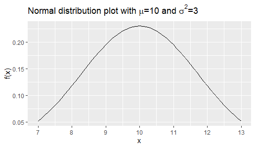
Now let us consider a numeric example. Let’s say that we would like to sample from the normal distribution with mean 10 and variance 3 (represented by $\mathcal{N}(10,3)$ ). Using both methods, we will get a sample of 100, 1000 and 10,000 readings and plot the histogram. First let us show the graph of the density function of $\mathcal{N}(10,3)$ . We will compare the shape of the sample histograms to the shape of this probability density function.

The following is the R code for a Monte Carlo Simulation. It accepts $n$ which is the sample size as its input. The function $runif(n,0,1)$ generates $n$ uniformly distributed random numbers. The function $qnorm$ is the inverse cumulative distribution function $F^{-1}$ which converts the uniformly distributed numbers to our final sample. It displays a histogram of this sample as its output.

#Monte Carlo Simulation

n<-1000 #sample size
Sample<-qnorm(runif(n,0,1),mean = 10, sd = sqrt(3))
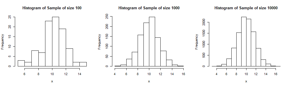
hist(Sample,main=paste("Histogram of Sample of size",as.character(n)))

We obtain 3 histograms for samples of sizes 100, 1000 and 10,000 respectively. We see that as the sample size increases, the shape of the histogram becomes more symmetric and near to the theoretic shape of the normal distribution $\mathcal{N}(10,3)$ .

The following is a code for a Latin Hypercube Simulation. It is similar to the one for MCS. However here the interval [0,1] is divided into $n$ portions and a number is sampled randomly from each interval. This is done through the $for$ loop. Again these numbers are transformed using the $qnorm$ function to give our required sample.

n<-1000

U<-c()
for (i in 1:n)
{U<-c(U,runif(1,(i-1)/n,i/n))}

Sample<-qnorm(U,mean = 10, sd = sqrt(3))
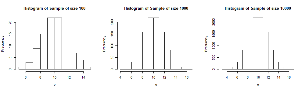
hist(Sample,xlab="x",main=paste("Histogram of Sample of size",as.character(n)))

Here we display 3 histograms for samples of sizes 100, 1000 and 10,000 respectively. We see, especially when compared to the output of the MCS, that these histogram have a more symmetric shape (and thus more similar to the shape of $\mathcal{N}(10,3)$ ), even for a sample size of just 100.

Convergence of MCS and LHS

We already have a hint that the LHS provides a more representative sample than the MCS. Now let us analyse in more detail the convergence of these two sampling methods. We will study the convergence of the sample mean and sample standard deviation to the values of the true parameters, for both methods.

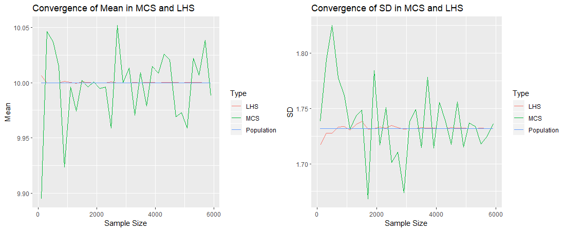
For each method, let us obtain samples of increasing size and compute their means and standard deviations, and see by how much they deviate from $\mu=10$ and $\sigma=\sqrt{3}\simeq 1.73$ . Consider the plot on the left corresponding to the mean. The blue line represents $\mu=10$ . The red line (corresponding to the Latin Hypercube samples) is very near to the mean. Even with a sample size of say 400, we obtain a sample mean so close to the true mean. The green line (corresponding to the Monte Carlo samples), even though it oscillates around the true mean, does not get so much close. Similarly, the plot on the right shows that the standard deviation of the Latin Hypercube samples converges much faster to the true standard deviation, than that of the Monte Carlo samples. One can say that a sample of size 400 using LHS is a more representative sample than a Monte Carlo sample of size 6,000.

The advantage of LHS over MCS is that you need a much lower sample size in order to obtain some particular precision. Since the computational time is directly proportional to the number of iterations, when using LHS in modelling, one would obtain the output much quicker. When working with huge data, this might mean that you obtain a result in 1 hour instead of 1 day, or makes a computation feasible instead of infeasible, for example.

Generalisation of the MCS and LHS to the bivariate case

Suppose now that we have two variables $X_1$ and $X_2$ , having a joint probability density function $f(x_1,x_2)$ and we would like to obtain a sample of $n$ data points where each data point is an ordered pair of the form $(x_1,x_2)$ where $x_1$ is a realisation of $X_1$ and $x_2$ is a realisation of $X_2$ .

Bivariate MCS

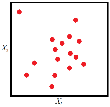
Recall that in the univariate case we choose $n$ random points of $X$ such that the shape of the sample histogram is similar to the shape of the probability density function. In the bivariate case we choose $n$ random points of $(X_1,X_2)$ such that the bivariate histogram (which could be displayed as a 3D-histogram) of the sample has a shape similar to that of the joint probability density function. The next figure shows the plane made up of all possible values of $X_1$ and $X_2$ . The red points make up a sample whose histogram would converge to the joint probability density function as $n\rightarrow\infty$ .

MCS is performed as follows. The function $f(x_1,x_2)$ could be written as:

$\begin{equation*} f(x_1,x_2)=g(x_1)h(x_2|x_1) \end{equation*}$

where $g(x_1)$ is the marginal density function of $X_1$ and $h(x_2|x_1)$ is the conditional density function of $X_2$ given $X_1$ . Equivalently, $f(x_1,x_2)$ can be written as:

$\begin{equation*} f(x_1,x_2)=g(x_2)h(x_1|x_2) \end{equation*}$

where $g(x_2)$ is the marginal distribution of $X_2$ and $h(x_1|x_2)$ is the conditional distribution of $X_1$ given $X_2$ . Either of the two equations could be used to implement MCS. However these determine which variable is chosen first. Without any loss of generality, let us use the first equation $f(x_1,x_2)=g(x_1)h(x_2|x_1)$ . Hence in MCS, first a value for $X_1$ is chosen and then a value for $X_2$ is chosen, depending on the realisation of $X_1$ . Same as in the univariate MCS, we make use of the Analytical Inversion Method. This time two uniformly distributed random variables $u_1$ and $u_2$ are generated. Then $x_1$ , the realisation of $X_1$ , is obtained by the equation $x_1=G^{-1}(u_1)$ , where $G^{-1}$ is the inverse marginal cumulative distribution function of $X_1$ . The value $x_2$ is obtained by using the equation $x_2=H^{-1}(u_2)$ where $H^{-1}$ is the inverse conditional cumulative distribution function of $X_2$ given $X_1=x_1$ . Thus we have our first sample point, which is the ordered pair $(x_1,x_2)$ . This process is repeated $n$ times in order to obtain a sample of size $n$ .

In the case where $X_1$ and $X_2$ are independent, the process is simplified as follows. We have:

$\begin{equation*} f(x_1,x_2)=g(x_1)h(x_2) \end{equation*}$

where $g(x_1)$ is the marginal density function of $X_1$ and $h(x_2)$ is the marginal density function of $X_2$ . Two uniformly distributed random variables $u_1$ and $u_2$ are generated. The realisation of $X_1$ is obtained by the equation $x_1=G^{-1}(u_1)$ , where $G^{-1}$ is the inverse marginal cumulative distribution function of $X_1$ and the value $x_2$ is obtained by using the equation $x_2=H^{-1}(u_2)$ where $H^{-1}$ is the inverse marginal cumulative distribution function of $X_2$ . This process is repeated $n$ times in order to obtain a sample of $n$ ordered pairs.

Bivariate LHS

Let us assume that the random variables $X_1$ and $X_2$ are independent. Now let’s consider the space of all possible values of $X_1$ and $X_2$ . In LHS, this space is transformed into a grid that results in the space being broken down into $n^2$ subspaces. The volume under the curve $f(x_1,x_2)$ bound by a subspace is $\frac{1}{n^2}$ . Thus this grid breaks down the volume under the curve, into $n^2$ portions, all having an equal volume of $\frac{1}{n^2}$ . Let the grid lines be $X_1=a_0,a_1,a_2,\cdots,a_n$ (where $a_0<a_1<a_2<\cdots<a_n$ ) and $X_2=b_0,b_1,b_2,\cdots,b_n$ (where $b_0<b_1<b_2<\cdots<b_n$ ). Then:

$\begin{equation*} \int_{b_{j-1}}^{b_j}\int_{a_{i-1}}^{a_i} f(x_1,x_2) dx_1dx_2=\frac{1}{n^2}, \end{equation*}$

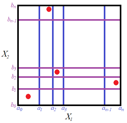
for all $i =1,2,\cdots,n$ and $j=1,2,\cdots,n$ . In LHS $n$ subspaces are chosen from the $n^2$ subspaces such that no two subspaces lie on the same row or column of the grid.

The gridded sample space looks like the following diagram. The red points give an example of a possible sample.

The random variable $F_1(X_1)$ , where $F_1$ is the (marginal) cumulative distribution of $X_1$ , follows the uniform distribution on the interval $[0,1]$ . We have seen this when describing the Analytical Inversion Method for the univariate case. Similarly the random variable $F_2(X_2)$ , where $F_2$ is the (marginal) cumulative distribution of $X_2$ , follows the uniform distribution on the interval $[0,1]$ . Now since $X_1$ and $X_2$ are independent, the joint distribution of $X_1$ and $X_2$ could be transformed into a joint uniform distribution with independent variables $F_1(X_1)$ and $F_1(X_2)$ which we shall call them $U_1$ and $U_2$ . Now the gridded sample space of $(X_1,X_2)$ is transformed into the following sample space of $(F_1(X_1),F_2(X_2))=(U_1,U_2)$ .

Here we see that the grid is now made up of perfect squares. Thus the volume under the bivariate uniform distribution is split into $n^2$ cubes each have a volume of $\frac{1}{n^2}$ . The gridlines of the two sample spaces are linked by the following equation: $F_1(a_0)=0, F_1(a_1)=\frac{1}{n}, F_1(a_2)=\frac{2}{n},\cdots,F_1(a_n)=1$ and $F_2(b_0)=0, F_2(b_1)=\frac{1}{n}, F_2(b_2)=\frac{2}{n},\cdots,F_2(b_n)=1$ .

The bivariate LHS method goes as follows. A sample of $n$ variables $u^{'}_{11},u^{'}_{12},\cdots,u^{'}_{1n}$ are chosen randomly from the intervals $[0,\frac{1}{n}], [\frac{1}{n},\frac{2}{n}],\cdots,[\frac{n-1}{n},1]$ respectively. A sample of $n$ variables labelled $u^{'}_{21},u^{'}_{22},\cdots,u^{'}_{2n}$ are chosen randomly from the intervals $[0,\frac{1}{n}], [\frac{1}{n},\frac{2}{n}],\cdots,[\frac{n-1}{n},1]$ respectively. Note that the two sequences $u^{'}_{11},u^{'}_{12},\cdots,u^{'}_{1n}$ and $u^{'}_{21},u^{'}_{22},\cdots,u^{'}_{2n}$ are increasing sequences. Let the sequence $u^{'}_{11},u^{'}_{12},\cdots,u^{'}_{1n}$ be shuffled randomly resulting in the sequence $u_{11},u_{12},\cdots,u_{1n}$ . Similarly, let the sequence $u^{'}_{21},u^{'}_{22},\cdots,u^{'}_{2n}$ be shuffled randomly resulting in the sequence $u_{21},u_{22},\cdots,u_{2n}$ . The resultant two sequences are combined in the sample $(u_{11},u_{21}),(u_{12},u_{22}),\cdots,(u_{1n},u_{2n})$ . Note that these are represented by the red dots in the diagram for the sample space of $(U_1,U_2)$ . Finally this is transformed to $(F_1^{-1}(u_{11}),F_2^{-1}(u_{21})),(F_1^{-1}(u_{12}),F_2^{-1}(u_{22})),\cdots,(F_1^{-1}(u_{1n}), F_2^{-1}(u_{2n}))$ which would be a Latin Hypercube sample from the sample space of $(X_1,X_2)$ . This is represented by the red dots in the diagram of the sample space of $(X_1,X_2)$ .

Note that in the general case when the two random variables are not independent, one must find a transformation from these variables into two independent ones and then carry on with the procedure for LHS. In fact the Cholesky decomposition can be used to transform $n$ correlated random variables into $n$ uncorrelated random variables (which are linear combinations of the correlated ones). In the case of normally distributed random variables, since their linear combinations are still normally distributed, then the Cholesky decomposition results in a multivariate normal distribution with an identity correlation matrix.

Example: Sampling from the bivariate normal with marginals $\mathcal{N}(2,4)$ and $\mathcal{N}(3,1)$ with correlation 0.

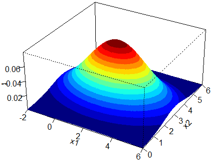
We will use both methods to obtain a sample of 1,000, 10,000 and 100,000 readings from this bivariate normal distribution. First let us display the 3D plot of this distribution and its associated contour plot. For an in-depth article on the structure and construction of contour plots and 3D plots of bivariate normal distributions click here.

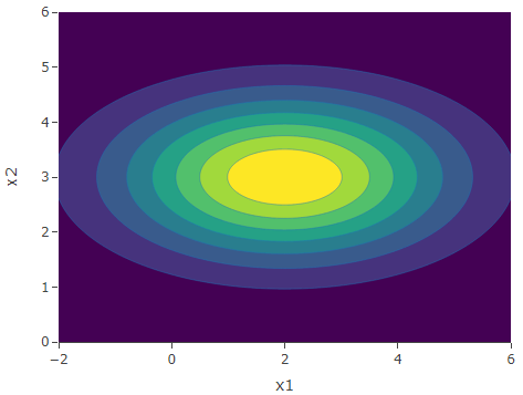
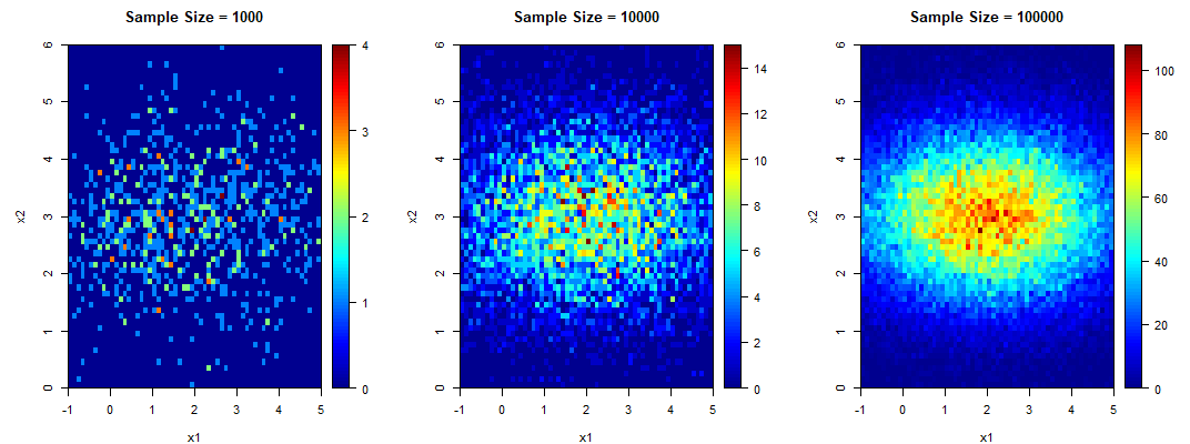
We will compare the shape of the sample contour plots to that of the population. The following is the code for MCS which produces a sample contour plot for sample size $n$ .

#bivariate MCS
library(plot3D)

n<-10000 #sample size

u1<-runif(n)
u2<-runif(n)

x1<-qnorm(u1,2,2) #converting to normal distribution with mean 2 sd 2
x2<-qnorm(u2,3,1) #converting to normal distribution with mean 3 sd 1

x1c<-cut(x1,seq(-1,5,0.1))
x2c<-cut(x2,seq(0,6,0.1))
z<-table(x1c, x2c)
image2D(z=z,seq(-1,5,0.1),seq(0,6,0.1),xlab="x1",ylab="x2",main=paste("Sample Size =",as.character(n)))

The following are the sample contour plots for $n=1000, 10000$ and 100000. We see the convergence of the sample contour plots to the population contour plot.

The following is the code for bivariate LHS which similarly produces a sample contour plot for sample size $n$ .

#bivariate LHS
library(plot3D)

n<-10000 #sample size

U1<-c()
for (i in 1:n)
{U1<-c(U1,runif(1,(i-1)/n,i/n))}
U1<-sample(U1)
x1<-qnorm(U1,2,2) #converting to normal distribution with mean 2 sd 2

U2<-c()
for (i in 1:n)
{U2<-c(U2,runif(1,(i-1)/n,i/n))}
U2<-sample(U2)
x2<-qnorm(U2,3,1) #converting to normal distribution with mean 3 sd 1

x1c<-cut(x1,seq(-1,5,0.1))
x2c<-cut(x2,seq(0,6,0.1))
z<-table(x1c, x2c)
image2D(z=z,seq(-1,5,0.1),seq(0,6,0.1),xlab="x1",ylab="x2",main=paste("Sample Size =",as.character(n)))

The following are the sample contour plots for $n=1000, 10000$ and 100000.

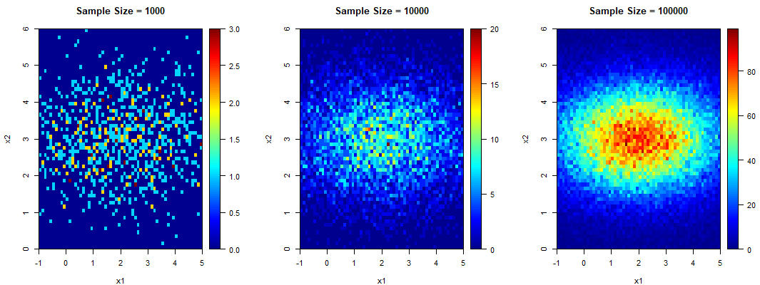
The contour plots for the LHS seem to be slightly more defined than those for the MCS. However the difference is not clear enough from these plots. Hence let us have a more detailed look at the convergence of both methods.

Convergence of the bivariate MCS and LHS

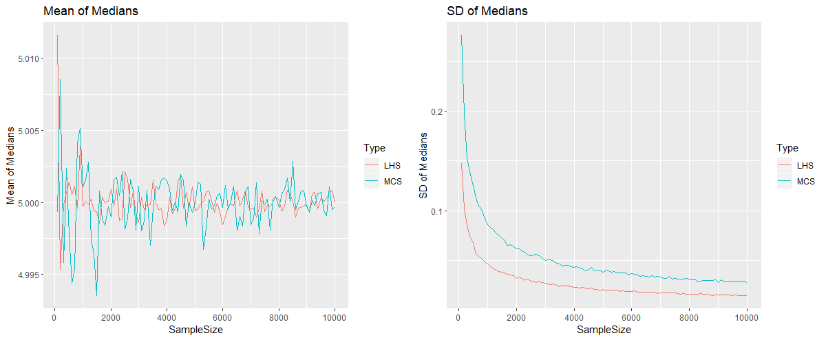
Suppose that we are interested in the median value of $X_1+X_2$ . Theoretically we know that this is equal to 5, but let us have a look at the performance of each sampling method. For each method, a sample of 100 readings (pairs of $X_1$ and $X_2$ ) is gathered and the sample median of $X_1+X_2$ is calculated. This is repeated for 1,000 times (since 1,000 simulations were carried out). Hence we have a sample of 1,000 sample medians of $X_1+X_2$ , for which we compute their mean and standard deviation. All this procedure is repeated for samples of 200, 300 up to 10,000 readings. We obtain the following plots. The mean of the medians oscillate around 5, for both methods. When we look at the plot for the standard deviation, we see that the output from the Latin Hypercube Simulation has less variance than the output from the Monte Carlo Simulation, for any sample size. In fact here the output from the LHS with 2,500 iterations has more or less the same variation as the output from MCS with 10,000 iterations. The code that performs the simulations and produces these diagrams, which is quite lengthy is provided in the appendix below.

Conclusion

We have seen the process of obtaining Monte Carlo Samples and Latin Hypercube Samples in both univariate and bivariate cases. We have seen with the help of examples that LHS produces results that have less variability that MCS, for any given number of iterations. MCS is a very simple idea to implement and even its associated code is very short, however LHS can produce the same quality of results with less computational time needed. These two sampling techniques could be extended to the multivariate cases in similar fashion.

Appendix

The following is the code that compares the output and variability of MCS and LHS for sample sizes $100, 200, \cdots, 10,000$ over 1,000 simulations.

library(ggplot2)
library(cowplot)

#MCS

N<-1000

MedianDataMC<-data.frame()

for(i in 1:N)
{
  medianxPyMC<-c()
  
  for (n in seq(100,10000,100))
  {
    u<-runif(n)
    v<-runif(n)
    
    x<-qnorm(u,2,2)
    y<-qnorm(v,3,1)
    
    medianxPyMC<-c(medianxPyMC,median(x+y))
    
  }
  MedianDataMC<-rbind(MedianDataMC,medianxPyMC)
}

#LHS

N<-1000

MedianDataLH<-data.frame()

for(i in 1:N)
{
  medianxPyLH<-c()
  
  for (n in seq(100,10000,100))
  {
    u<-c()
    for (i in 1:n)
    {u<-c(u,runif(1,(i-1)/n,i/n))}
    u<-sample(u)
    
    v<-c()
    for (i in 1:n)
    {v<-c(v,runif(1,(i-1)/n,i/n))}
    v<-sample(v)
    
    x<-qnorm(u,2,2)
    y<-qnorm(v,3,1)
    
    medianxPyLH<-c(medianxPyLH,median(x+y))
  }
  MedianDataLH<-rbind(MedianDataLH,medianxPyLH)
}

MeanOfMediansMC<-c()
for(i in 1:ncol(MedianDataMC)){MeanOfMediansMC<-c(MeanOfMediansMC,mean(MedianDataMC[,i]))}
SDOfMediansMC<-c()
for(i in 1:ncol(MedianDataMC)){SDOfMediansMC<-c(SDOfMediansMC,sd(MedianDataMC[,i]))}

MeanOfMediansLH<-c()
for(i in 1:ncol(MedianDataLH)){MeanOfMediansLH<-c(MeanOfMediansLH,mean(MedianDataLH[,i]))}
SDOfMediansLH<-c()
for(i in 1:ncol(MedianDataLH)){SDOfMediansLH<-c(SDOfMediansLH,sd(MedianDataLH[,i]))}

Data<-data.frame(SampleSize=c(seq(100,10000,100),seq(100,10000,100)),MeanOfMedians=c(MeanOfMediansMC,MeanOfMediansLH),SDOfMedians=c(SDOfMediansMC,SDOfMediansLH),Type=c(rep("MCS",length(seq(100,10000,100))),rep("LHS",length(seq(100,10000,100)))))

plot1<-ggplot() + geom_line(data = Data, aes(x = SampleSize, y = MeanOfMedians, color = Type))+ scale_x_continuous(breaks = seq(0,10000,by=2000))+ylab("Mean of Medians")+ggtitle("Mean of Medians")
plot2<-ggplot() + geom_line(data = Data, aes(x = SampleSize, y = SDOfMedians, color = Type))+ scale_x_continuous(breaks = seq(0,10000,by=2000))+ylab("SD of Medians")+ggtitle("SD of Medians")

plot_grid(plot1, plot2)