Different Correlation Structures in Copulas

DIfferent Correlation Structures In Copulas

Introduction

Copulas are used to combined a number of univariate distributions into one multivariate distribution. Different copulas will describe the correlation structure between the variables in various ways. For example the multivariate normal distribution results from using a copula named the “Gaussian” copula on marginal univariate normal distributions. However there a number of other copulas that can be used to “join” univariate distributions, in a way that define the correlation structure in a non-uniform fashion. We will look into some of the most commonly used copulas and see how they differ in the way they model the correlation structure. We will analyse the contour plots of bivariate distributions constructed from different copulas over the same two marginal distribution functions.

What is a copula?

An $n$ -dimensional copula $C$ is multivariate cumulative distribution function on $n$ marginal uniformly distributed random variables $U_1,U_2,\cdots,U_n$ each having domain [0,1]. Hence a copula determines/describes the correlation structure between these $n$ uniformly distributed random variables. In 1959, Abe Sklar showed that any cumulative multivariate distribution can be expressed a function of a copula and its marginal distributions. This is done as follows. Suppose that we have $n$ continuous random variables $X_1,X_2,\cdots,X_n$ with cumulative distribution functions $F_1,F_2,\cdots,F_n$ respectively. Using some algebra it can be that the random variables $F_1(X_1),F_2(X_2),\cdots, F_n(X_n)$ are uniformly distributed. The cumulative multivariate distribution function can be expressed as:

$\begin{equation*} F(x_1,x_2,\cdots,x_n)=C(F_1(x_1),F_2(x_2),\cdots, F_n(x_n)) \end{equation*}$

By differentiating w.r.t. $x_1,x_2,\cdots,x_n$ , we obtain the multivariate density function:

$\begin{equation*} f(x_1,x_2,\cdots,x_n)=c(F_1(x_1),F_2(x_2),\cdots, F_n(x_n))f_1(x_1)f_2(x_2)\cdots f_n(x_n), \end{equation*}$

where $f_1,f_2,\cdots, f_n$ are the marginal probability density functions of $X_1,X_2,\cdots, X_n$ respectively. In the bivariate case the joint cumulative distribution function and the joint density function reduce to the form:

$\begin{equation*} F(x_1,x_2)=C(F_1(x_1),F_2(x_2))\mbox{ and }f(x_1,x_2)=c(F_1(x_1),F_2(x_2))f_1(x_1)f_2(x_2) \end{equation*}$

Let us consider the equations for the copulas in the bivariate case.

Gaussian Copula

For simplicity, let $u$ denote $F_1(x_1)$ and $v$ denote $F_2(x_2)$ . The bivariate Gaussian copula density function is given by:

$\begin{equation*} c(u,v)=\frac{1}{\sqrt{1-\rho^2}}\mbox{exp}\lbrace -\frac{1}{2}(\frac{1}{1-\rho^2}-1)(\Phi^{-1}(u)^2+\Phi^{-1}(v)^2)+\frac{\rho}{1-\rho^2}\Phi^{-1}(u)\Phi^{-1}(v)\rbrace. \end{equation*}$

Thus the joint probability density function becomes:

$\begin{equation*} f(x_1,x_2)=c(u,v)f_1(x_1)f_2(x_2). \end{equation*}$

Hence by knowing the two marginal cumulative distribution functions $F_1$ and $F_2$ and the correlation value between them $\rho$ , these are inserted in the function $c(u,v)$ and multiplied with the marginal densities to obtain the bivariate distribution. In particular, suppose that $X_1\sim\mathcal{N}(\mu_1,\sigma_1^2)$ and $X_2\sim\mathcal{N}(\mu_2,\sigma_2^2)$ . Then:

$\begin{equation*} \Phi^{-1}(u)=\Phi^{-1}(F_1(x_1))=\Phi^{-1}(\Phi(\frac{x_1-\mu_1}{\sigma_1}))=\frac{x_1-\mu_1}{\sigma_1}. \end{equation*}$

Similarly: $\Phi^{-1}(v)=\frac{x_2-\mu_2}{\sigma_2}$ . In this case, the copula density function becomes:

$\begin{equation*} c(u,v)=\frac{1}{\sqrt{1-\rho^2}}\mbox{exp}\lbrace -\frac{1}{2}(\frac{1}{1-\rho^2}-1)(\frac{(x_1-\mu_1)^2}{\sigma_1^2}+\frac{(x_2-\mu_2)^2}{\sigma_2^2})+\frac{\rho(x_1-\mu_1)(x_2-\mu_2)}{(1-\rho^2)\sigma_1\sigma_2}\rbrace. \end{equation*}$

Thus,

$\begin{equation*} \begin{split} f(x_1,x_2)&=c(u,v)f_1(x_1)f_2(x_2)\\ &=\frac{1}{\sqrt{1-\rho^2}}\mbox{exp}\lbrace -\frac{1}{2}(\frac{1}{1-\rho^2}-1)(\frac{(x_1-\mu_1)^2}{\sigma_1^2}+\frac{(x_2-\mu_2)^2}{\sigma_2^2})+\frac{\rho(x_1-\mu_1)(x_2-\mu_2)}{(1-\rho^2)\sigma_1\sigma_2}\rbrace \frac{1}{\sqrt{2\pi\sigma_1^2}}\mbox{exp}\lbrace-\frac{(x_1-\mu_1)^2}{2\sigma_1^2}\rbrace\frac{1}{\sqrt{2\pi\sigma_2^2}}\mbox{exp}\lbrace-\frac{(x_2-\mu_2)^2}{2\sigma_2^2}\rbrace\\ &=\frac{1}{2\pi\sigma_1\sigma_2\sqrt{1-\rho^2}}\mbox{exp}\lbrace -\frac{1}{2}(\frac{1}{1-\rho^2})(\frac{(x_1-\mu_1)^2}{\sigma_1^2}+\frac{(x_2-\mu_2)^2}{\sigma_2^2})+\frac{\rho(x_1-\mu_1)(x_2-\mu_2)}{(1-\rho^2)\sigma_1\sigma_2}\rbrace \end{split} \end{equation*}$

This is in fact the equation of the bivariate normal distribution. In general, using the Gaussian copula on marginal normal distributions results in the multivariate normal distribution.

As an example let $X_1 X_2\sim\mathcal{N}(0,1)$ . Let consider their joint probability density function using the Gaussian copula with $\rho=-0.7, 0$ and 0.4. The following R code gives us the contour plot of $f(x_1,x_2)$ . Note that a contour plot is a representation of a 3D plot on 2D surface. The two dimensions represent $X_1$ and $X_2$ . The pairs $(x_{11},x_{21})$ and $(x_{12},x_{22})$ have the same colour if they have the same $f$ value $f(x_{11},x_{21})=f(x_{12},x_{22})$ . A contour is a group of points having the same colour (i.e. the same $f$ value).

We will use two packages: “copula” in order to use functions that built a multivariate distribution from a copula and two marginal distributions, and “plotly” which displays the contour plot. The variable “rho” is the input, which could take any value from the interval (-1,1). In this case the function “mvdc” constructs the bivariate distribution from the Gaussian copula and two standard normal marginal distributions. The sequences “x1” and “x2” define the sample domain of $X_1$ and $X_2$ for the contour plot. The matrix $f$ is made up of the values of the bivariate density function for the elements of the cross product of “x1” and “x2”.

library(copula)
library(plotly)

#Normal Copula

rho<-0.4

Normal_Cop<-mvdc(normalCopula(rho,dim = 2), margins=c("norm","norm"),
     paramMargins=list(list(mean=0, sd=1),list(mean=0, sd=1)))

x1 <- x2 <- seq(-3, 3, length= 100)

v<-c()
for (i in x1)
{for (j in x2){v<-c(v,dMvdc(c(i,j), Normal_Cop))}}
f<-t(matrix(v,nrow=100,byrow=TRUE))

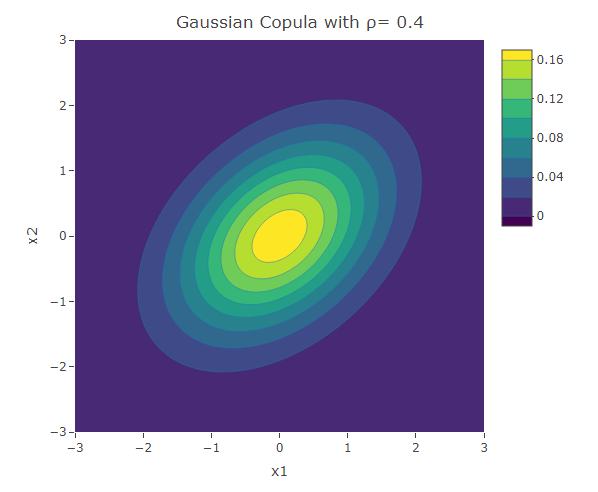
plot_ly(x=x1,y=x2,z=f,type = "contour")%>%layout(xaxis=list(title="x1"),yaxis=list(title="x2"),title=paste("Gaussian Copula with ρ=",as.character(rho)))

The following are three plots of the bivariate distribution with the Gaussian copula for $\rho=-0.7,0$ and 0.4. The resultant contours have an elliptical shape.

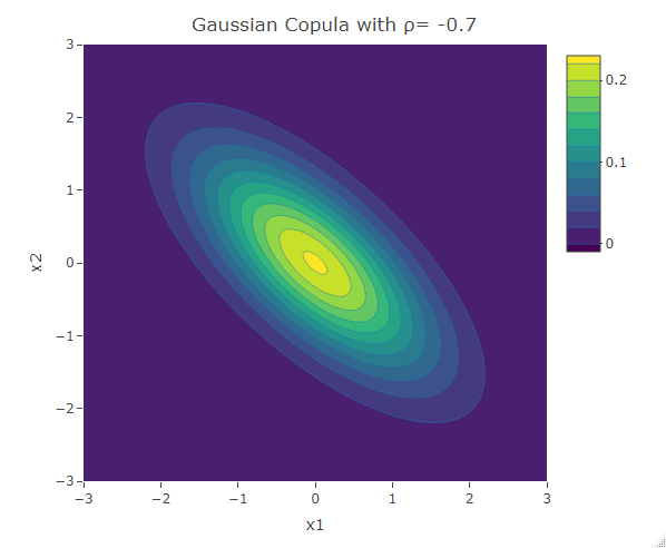
The contour plot resulting from the Gaussian copula with $\rho=0.4$ is symmetric about the line $x_2=-x_1$ . Thus the dependence structure in negative tail is the same as the dependence structure in the positive tail. Similar analysis can be done on the contour plot of a bivariate normal distribution for any feasible value of $\rho$ . This result from the elliptical structure of the contours. A higher correlation magnitude results in elliptical contours having a shorter length (along the second diagonal ), and vice-versa. For a more in-depth study of the structure of the bivariate normal distribution, click here.

Clayton copula

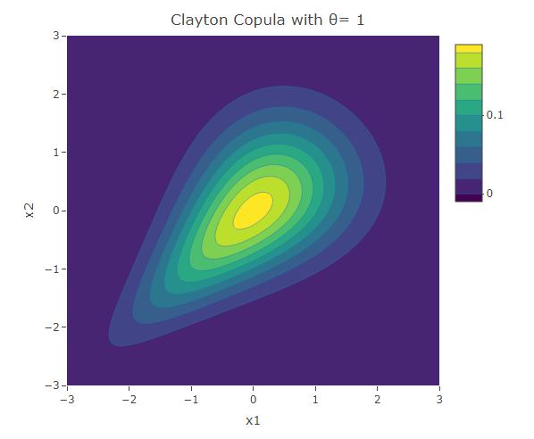
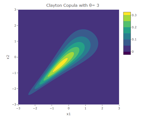
In the Clayton copula, there is more dependence in the negative tail than in the positive tails. Hence this is useful to model variables that become more correlated in a stress scenario. For example in finance one could observe more dependence in negative stock prices returns of two assets. In fact assuming a uniform dependence structure, as in the Gaussian copula, might lead to an underestimation of portfolio risk. The bivariate Clayton copula density function is given by:

$\begin{equation*} c(u,v)=(1+\theta)(uv)^{-1-\theta}(-1+u^{-\theta}+v^{-\theta})^{-2-\frac{1}{\theta}},\mbox{ for }\theta> 0. \end{equation*}$

Note that in the study of copulas, we usually use another common measure of correlation in place of the Pearson’s (linear) correlation $\rho$ . This is Kendall’s tau $\tau$ , which quantifies the relationship between two variables by the ranking of their values. Note that the ranking of the values of a random variable $X$ is the same as the ranking of the values of the random variable g(X) if $g$ is an increasing function. Since both $F_1$ and $F_2$ are increasing functions, Kendall’s $\tau$ depends on the copula’s parameter and not on the marginal distributions. Hence any appropriate marginal distributions used will give the same $\tau$ value. For the Clayton copula $\tau=\frac{\theta}{\theta+2}$ . Thus $\tau$ is positive for the Clayton copula and increases with the value of $\tau$ .

#Clayton Copula

theta<-1

Clayton_Cop<- mvdc(claytonCopula(theta, dim = 2), margins=c("norm","norm"),
                    paramMargins=list(list(mean=0, sd=1),list(mean=0, sd=1)))

x1 <- x2 <- seq(-3, 3, length= 200)

v<-c()
for (i in x1)
{for (j in x2){v<-c(v,dMvdc(c(i,j), Clayton_Cop))}}
f<-t(matrix(v,nrow=200,byrow=TRUE))

plot_ly(x=x1,y=x2,z=f,type = "contour")%>%layout(xaxis=list(title="x1"),yaxis=list(title="x2"),title=paste("Clayton Copula with θ=",as.character(theta)))

The following are three plots of the bivariate distribution with Clayton copula for $\theta= 1,2$ and 3. We see that the width of the contours decrease with the increase in the value of $\theta$ , indicating the increase in the correlation. Due to the asymmetric structure, one can see that the negative tails are more dependent than the positive tails.

Gumbel Copula

The bivariate Gumbel copula density function is given by:

$\begin{equation*} c(u,v)=\frac{1}{uv}[(\ln{u})(\ln{v})]^{\theta-1}C[(-\ln{u})^{\theta}+(-\ln{u})^{\theta}]^{\frac{1-2\theta}{\theta}}[\theta - 1 + ((-\ln{u})^{\theta}+(-\ln{u})^{\theta})^{\frac{1}{\theta}}]\mbox{ for }\theta\geq 1,\mbox{ where }C=e^{-[(-\ln{u})^{\theta}+(-\ln{u})^{\theta}]^{\frac{1}{\theta}}}. \end{equation*}$

Kendall’s Tau is $\tau=\frac{\theta-1}{\theta}$ . Hence, similar to the Clayton copula, this copula is defined for non-negative $\tau$ and the value of $\tau$ increases with the value of $\theta$ .

#Gumbel Copula

theta<-2

Gumbel_Cop<- mvdc(gumbelCopula(theta, dim = 2), margins=c("norm","norm"),
                 paramMargins=list(list(mean=0, sd=1),list(mean=0, sd=1)))

x1 <- x2 <- seq(-3, 3, length= 200)

v<-c()
for (i in x1)
{for (j in x2){v<-c(v,dMvdc(c(i,j), Gumbel_Cop))}}
f<-t(matrix(v,nrow=200,byrow=TRUE))

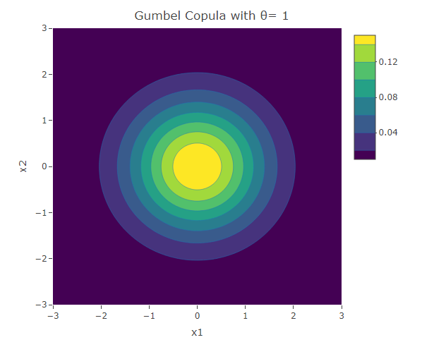
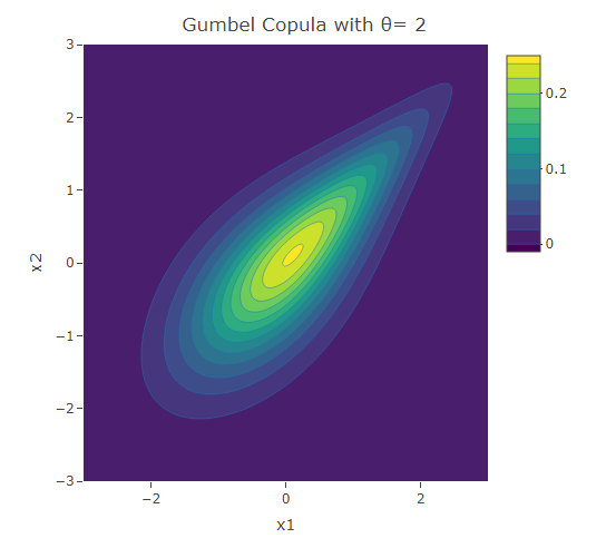
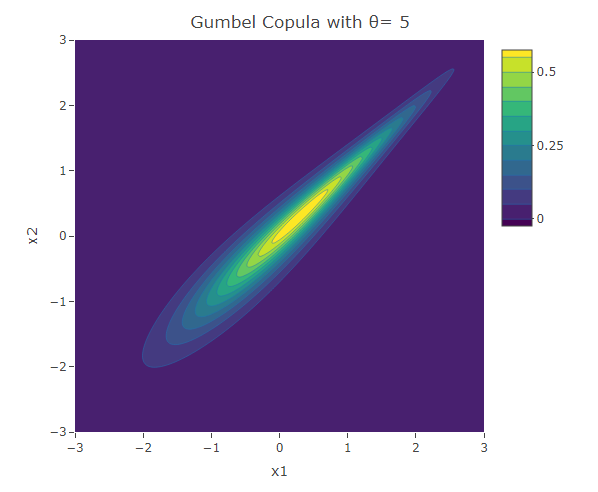
plot_ly(x=x1,y=x2,z=f,type = "contour")%>%layout(xaxis=list(title="x1"),yaxis=list(title="x2"),title=paste("Gumbel Copula with θ=",as.character(theta)))

The following are three plots of the bivariate distribution resulting from the Clayton copula for $\theta= 1,2$ and 5. The copula with $\theta =1$ gives the case when the variables are independent. In fact $\tau=0$ in this case. We have seen this bivariate distribution when we used the Gaussian Copula with $\rho=0$ . For the rest of the cases (when $\theta>1$ ), similar to those resulting from the Clayton copula, the contours have an asymmetric structure. However in contrast to the Clayton copula, here the dependence structure in the positive tail is stronger than that in the negative tail.

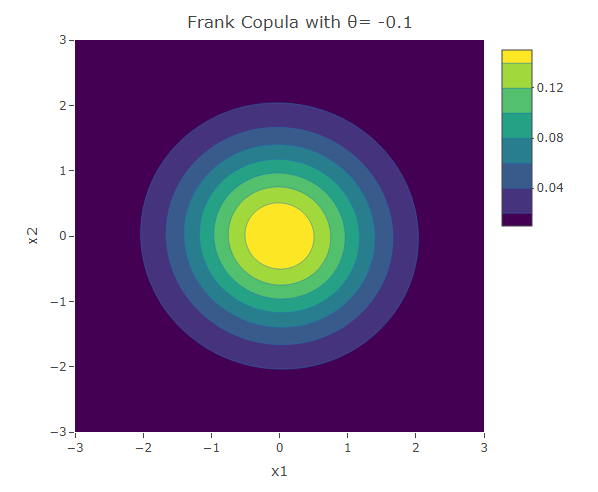
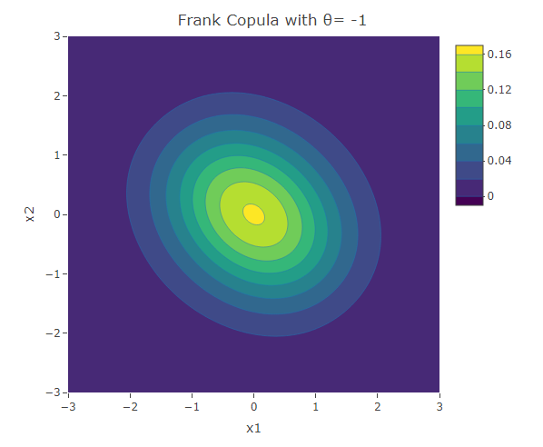
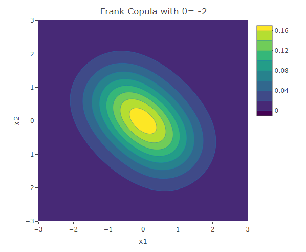
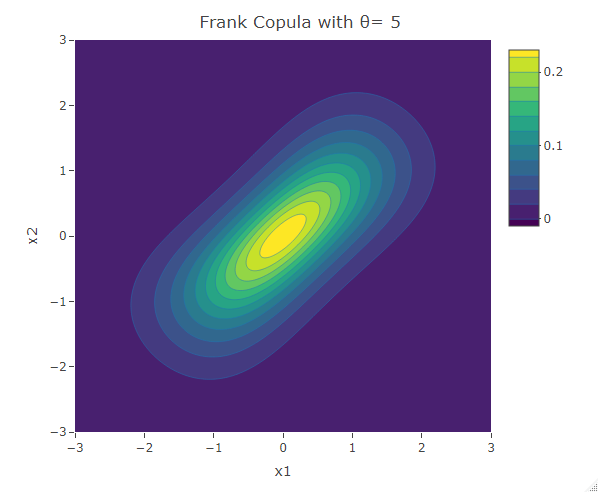
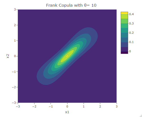
Frank Copula

Another common copula is the Frank copula. This provides a symmetric contour structure similar to the Gaussian copula. However with Frank copula, there is greater dependency in the tails (both positive and negative) than there is in the center. The bivariate Frank copula density function is given by:

$\begin{equation*} c(u,v)=\theta (e^{\theta}-1)\frac{e^{\theta (u+v)}}{[(e^{\theta u}-1)(e^{\theta v}-1)+(e^{\theta}-1)]^2}\mbox{ for }\theta\neq 0. \end{equation*}$

Kendall’s Tau for the Frank copula is $\tau=1+\frac{4}{\theta}[1+\frac{1}{\theta}\int_0^{-\theta} \frac{t}{e^t-1}dt]$ . The Frank copula is specified for both positive and negative correlation.

#Frank Copula

theta<-2

Frank_Cop<- mvdc(frankCopula(theta, dim = 2), margins=c("norm","norm"),
                   paramMargins=list(list(mean=0, sd=1),list(mean=0, sd=1)))

x1 <- x2 <- seq(-3, 3, length= 200)

v<-c()
for (i in x1)
{for (j in x2){v<-c(v,dMvdc(c(i,j), Frank_Cop))}}
f<-t(matrix(v,nrow=200,byrow=TRUE))

plot_ly(x=x1,y=x2,z=f,type = "contour")%>%layout(xaxis=list(title="x1"),yaxis=list(title="x2"),title=paste("Frank Copula with θ=",as.character(theta)))

The following are some contour plots from the Clayton copula using various values for $\theta$ . As $\theta$ reaches 0, the bivariate distribution converges to the independent bivariate normal distribution. Negative values of $\theta$ are related to negative correlation between the variables and on the other hand positive values of $\theta$ are related to positive correlation.

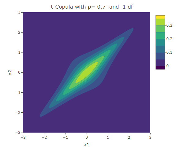
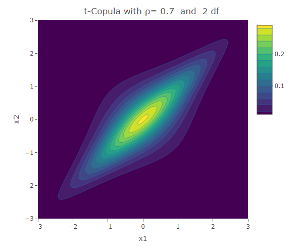
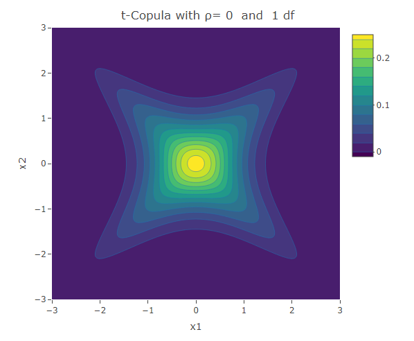
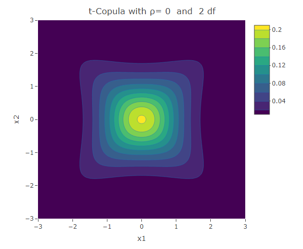
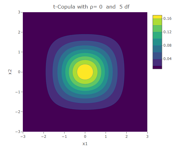
Student t-Copula

Similar to the Frank copula, in the Student t-Copula there is stronger dependence in the tails of the distribution. This copula has two parameters: $\rho$ the linear correlation coefficient and $d$ the degrees of freedom. The bivariate Student t-copula density function is given by:

$\begin{equation*} c(u,v)=\frac{\Gamma(0.5 d)\Gamma(0.5d+1)(1+\frac{t_d^{-2}(u)+t_d^{-2}(v)-2\rho t_d^{-1}(u)t_d^{-1}(v)}{d(1-\rho^2)})^{-\frac{d+2}{2}}}{\sqrt{1-\rho^2}\Gamma(0.5(d+1))^2(1+\frac{t^{-2}_d(u)}{d})^{-\frac{d+1}{2}}(1+\frac{t^{-2}_d(v)}{d})^{-\frac{d+1}{2}}}, \end{equation*}$

where $t^{-2}_d$ is the square of the inverse cumulative distribution function of the univariate student t-distribution with $d$ degrees of freedom. As $d$ increases, the Student t-copula converges to the Gaussian copula.

#t-Copula

rho<-0.7
df<-2

t_Cop<- mvdc(tCopula(rho, dim = 2,df=df), margins=c("norm","norm"),
               paramMargins=list(list(mean=0, sd=1),list(mean=0, sd=1)))

x1 <- x2 <- seq(-3, 3, length= 200)

v<-c()
for (i in x1)
{for (j in x2){v<-c(v,dMvdc(c(i,j), t_Cop))}}
f<-t(matrix(v,nrow=200,byrow=TRUE))

plot_ly(x=x1,y=x2,z=f,type = "contour")%>%layout(xaxis=list(title="x1"),yaxis=list(title="x2"),title=paste("t-Copula with ρ=",as.character(rho)," and ",as.character(df),"df"))

The following are some contour plots from the Student t-copula using various three values of $rho$ , namely -0.7, 0 and 0.4. We use increasing values of $d$ to show the convergence to the three contour plots presented for the Gaussian copula section.

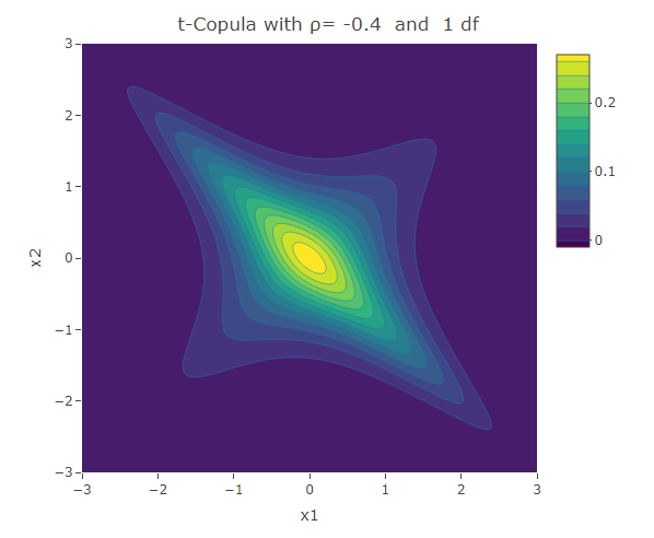
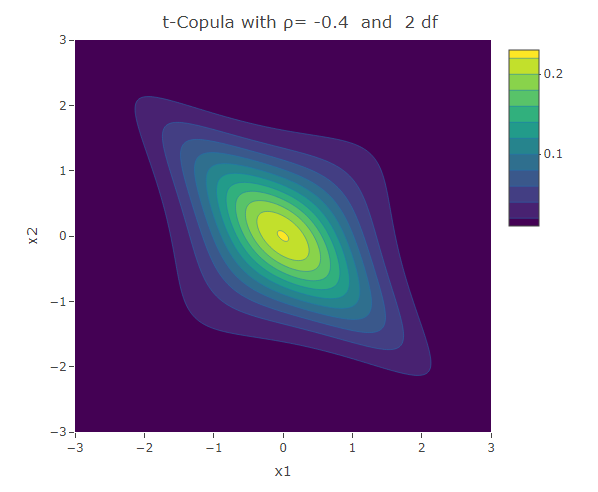
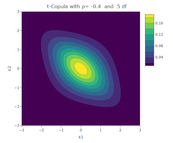
Conclusion

We have seen a number of different ways how two univariate distributions can be joined together to form a bivariate distribution. The different copulas have their own way how to describe the correlation structure between the variables. We have seen the Gaussian copula which is related to the multivariate normal distribution. However there are other copulas that could be used to model situations in which the correlation structure is not linear over the domain of its variables. The Clayton and Gumbel copula, result in asymmetric contours of their bivariate probability density function and have a stronger dependence structure in the negative and positive tail respectively. The Frank copula results in symmetric contours, however it has stronger dependence structure in both of its tails. The Student t-Copula is derived from the t-distribution. It has star-like contours and converges to the Gaussian copula as the number of degrees of freedom increases.